
Deep Learning Theory / DEEP LEARNING II
What One Replaced Example Changes: Algorithmic Stability, Training Time, and Generalization
A quantifier-aware account of data sensitivity, exact finite controls, and complete learning pipelines.
قد تتضمن ترجمة الذكاء الاصطناعي أخطاء. يُرجى التحقق بالرجوع إلى النص الأصلي.
النص الأصلي باللغة الإنجليزية. ترجمات هذه المراجعة الجديدة غير متاحة بعد.
Abstract
Algorithmic stability concerns the data-to-predictor procedure rather than architecture size alone. This review separates parameter, prediction, loss, average, uniform, and high-probability notions using six primary records. An exactly solvable regularized quadratic procedure gives explicit training trajectories, replacement-sensitivity bounds, and an expected generalization gap under a declared Rademacher distribution. The construction shows why low sensitivity can reflect not learning, and why an upper bound that grows with time is not itself an empirical test-error curve. We then examine data-dependent diagnostics, random coupling, adaptive selection, and scientifically meaningful sampling units. A proposed paired-retraining protocol retains sensitive cases and failed runs. The figures and enumeration are constructed controls, not new deep-network measurements or independent verification of the cited theorems.
In this paper
- 1. A training run is a data-dependent procedure
- 2. The selected papers do not use one interchangeable notion
- 3. Neighboring data and random coupling must be declared
- 4. Loss stability differs from parameter stability
- 5. A quadratic procedure with a closed-form trajectory
- 6. Replacing one observation yields an explicit sensitivity bound
- 7. Expected generalization can also be computed in one special distribution
- 8. A bound that worsens with time is not an empirical learning curve
- 9. Data-dependent quantities require their own statistical discipline
- 10. Expectation and tail guarantees answer different operational questions
- 11. The whole selection pipeline can destabilize a stable learner
- 12. A finite verification artifact with negative controls
- 13. A deep-learning experiment that can test a specific hypothesis
- 14. Stability is useful when its quantifiers remain visible
1. A training run is a data-dependent procedure
A model's architecture does not by itself determine how much its prediction changes when one training observation is replaced. Initialization, sample ordering, optimizer state, stopping rules, preprocessing, and model selection can all affect that sensitivity. Algorithmic stability studies the procedure that maps data into a predictor, rather than only the size of the class of functions it could represent.
This review asks what stability can establish about generalization and what an empirical sensitivity experiment cannot establish on its own. Six primary records distinguish uniform, average, data-dependent, optimization-dependent, and high-probability arguments. We construct an exactly solvable regularized quadratic learning problem to connect training time, replacement sensitivity, and an expected generalization gap. Its purpose is not to make a new claim about contemporary deep-network benchmarks. It shows why a statement that training longer worsens a bound is different from a statement that every longer run has worse test accuracy. A complete account must preserve that distinction while stating the neighboring-dataset convention, randomness coupling, loss range, and sampling assumptions that give a stability claim its meaning.
2. The selected papers do not use one interchangeable notion
Bousquet and Elisseeff formalize stability-based generalization arguments. Hardt, Recht, and Singer analyze stochastic gradient methods under explicit smoothness and Lipschitz assumptions. Kuzborskij and Lampert develop data-dependent stability analysis. Their different quantifiers and assumptions matter: a worst-case replacement guarantee and an average sensitivity under a data distribution are not the same certificate.
Charles and Papailiopoulos connect stability to convergence and geometry under conditions such as Polyak-Lojasiewicz or quadratic growth. Lei and Ying refine SGD analyses, including on-average model stability and relaxed assumptions. Feldman and Vondrak distinguish expectation bounds from high-probability guarantees for uniformly stable bounded-loss procedures. These results motivate a layered interpretation rather than a single slogan that fast training always generalizes. We use the identified definitions and scope from the original records, not their historical priority claims as current rankings. Source proofs are not independently verified, and the finite quadratic construction below is not a numerical reproduction of their neural-network or general optimization examples.
3. Neighboring data and random coupling must be declared
Let S and S' contain n observations and differ in one replacement. A learning algorithm A maps a dataset and random seed into a predictor. A uniform loss-stability claim bounds the change in loss on every allowed test observation when the neighboring dataset changes, with the treatment of algorithmic randomness specified. Removing one observation instead of replacing it changes the dataset size and can require a different statement.
For randomized procedures, reusing the same seed in a paired experiment can isolate sensitivity to the replaced observation. It does not by itself establish a worst-case guarantee over seeds or a distribution-free bound over all datasets. Using independent seeds estimates a different quantity that mixes data sensitivity with training randomness. Both can be useful if named correctly. In a neural pipeline, sample order, augmentation draws, dropout masks, and mixed-precision execution may need their own coupling conventions. A plot of output disagreement without these details is an observation about an experiment, not yet an algorithmic-stability certificate. The distinction is especially important when the most sensitive examples are rare and unlikely to appear in a small replacement sample.
4. Loss stability differs from parameter stability
Two parameter vectors can be far apart while representing the same function because of symmetries or redundant units. Conversely, a small parameter change can cause a large loss change if the loss or input norm is not controlled. A bound on Euclidean parameter distance becomes a loss bound only after a suitable Lipschitz or other continuity argument is justified over the relevant domain.
Prediction disagreement on a finite probe set is another distinct quantity. It can reveal a problem but does not establish a uniform bound over unobserved inputs. A classifier may retain its top-ranked label while its probability or margin changes substantially, so a zero disagreement rate can conceal meaningful sensitivity. The most informative experiment records several levels separately: parameter movement under an explicit alignment, functional change on held-out probes, loss change, and the resulting task metric. Theory can connect these levels under assumptions. Without that connection, one should not attach the same word stability to all of them and then transfer a theorem proved for one quantity to an empirically measured different quantity.
5. A quadratic procedure with a closed-form trajectory
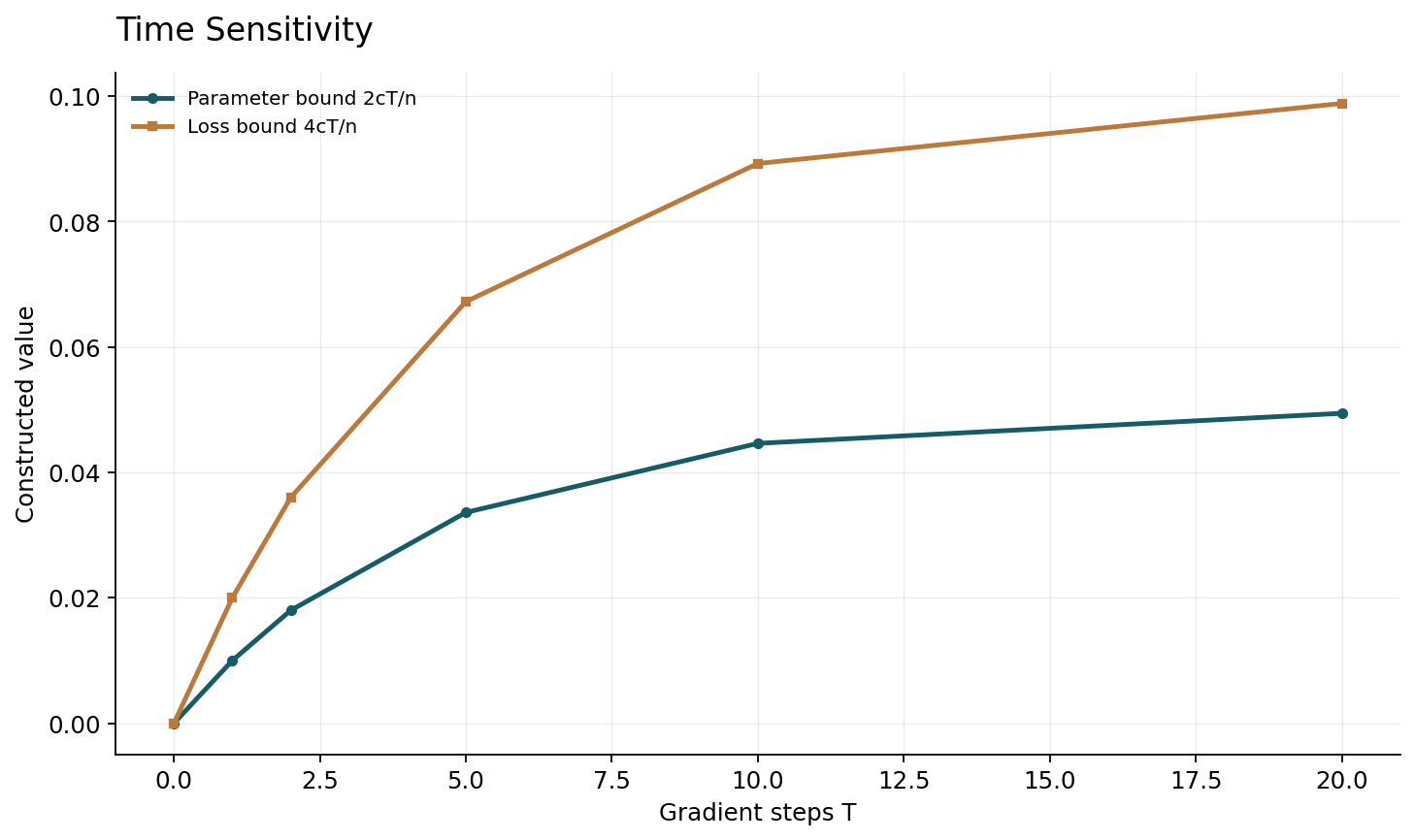
Consider scalar observations z in[-1,1], per-example loss one half of(w-z) squared, and regularization lambda times w squared divided by two, with lambda nonnegative. Full-batch gradient descent starts at zero with step eta satisfying0<eta<=1/(1+lambda). If m is the sample mean and q=1-eta(1+lambda), the update is w_next=q w+eta m. Solving this recurrence gives w_T=c_T m, with c_T=(1-q^T)/(1+lambda).
This model has bounded iterates and a transparent contraction factor. The loss normalization and regularization convention are part of its definition; changing either changes q and c_T. The construction uses deterministic full-batch updates rather than SGD, so it should not be presented as a direct verification of an SGD theorem. Its advantage is that every subsequent sensitivity and generalization calculation can be checked exactly. At T=0, the procedure ignores the data and has zero replacement sensitivity. As T increases, it uses more of the sample mean and approaches the regularized empirical minimizer. Whether this tradeoff improves the intended prediction task requires examining both approximation and estimation, not sensitivity alone.
6. Replacing one observation yields an explicit sensitivity bound
For replacement neighbors with observations in[-1,1], the sample means differ by at most2/n. The closed-form trajectory therefore gives |w_T(S)-w_T(S')|<=2c_T/n. Since w and z stay in[-1,1], the derivative of the squared loss with respect to w has absolute value at most two. A conservative uniform loss-difference bound is consequently4c_T/n for this declared model.
The factors have a clear interpretation. Increasing n reduces the influence of one observation; stronger regularization reduces the maximum c_T; training from zero for longer increases c_T toward its limit. None of this says that a predictor with the smallest c_T has the smallest risk. The procedure at T=0 is maximally insensitive because it has learned nothing. This is a useful negative control against an argument that treats low measured sensitivity as a sufficient performance objective. The bound is also conservative: a particular pair of neighboring datasets and probe point can have a substantially smaller loss difference. Reporting that smaller observation as the uniform constant would reverse the direction of the logical inference.
7. Expected generalization can also be computed in one special distribution
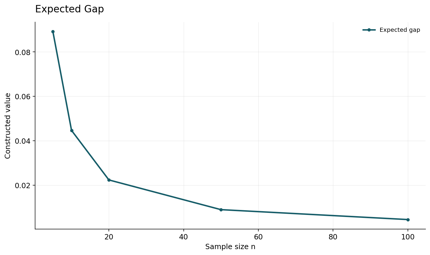
Let the observations now be independent Rademacher variables, taking values minus one and one with equal probability. The population mean is zero and the second moment is one. For the quadratic loss, population risk is one half of(w squared+1). Empirical risk is one half of(w squared-2wm+1), because every observed squared label equals one. Their difference is wm=c_T m squared.
Taking expectation over the sample gives an exact expected gap c_T/n, since the expected squared sample mean is1/n. This result is specific to the declared distribution and procedure. It is not a uniform high-probability statement or a formula for arbitrary deep networks. It does demonstrate an important separation: the expected gap can grow as the procedure learns more from data, while total risk also includes bias and the irreducible response variance. A generalization-gap bound is not automatically an excess-risk bound against the best predictor. Comparisons should retain the reference predictor, data-generating distribution, and sign convention for the gap so the object being estimated remains unambiguous.
8. A bound that worsens with time is not an empirical learning curve
A stability upper bound can increase with the number of updates because it accumulates worst-case effects. The actual test error on a given task can decrease, plateau, or increase. There is no contradiction: an upper bound is not a prediction of the observed curve unless a separate argument shows it is tight in the regime being studied.
The solvable model makes this distinction concrete. Increasing c_T raises the exact expected generalization gap under the chosen Rademacher distribution, yet under a different nonzero-mean distribution the zero predictor can have substantial bias. In that setting, some learning is necessary even though sensitivity increases. A stopping rule must therefore balance a task objective, not simply minimize a stability estimate. The inspected SGD records provide conditional results whose assumptions and conclusions should be read together. Turning a paper title about faster training into a universal prescription for early stopping discards both the optimization error and the sampling model that make the theorem informative.
9. Data-dependent quantities require their own statistical discipline
A data-dependent stability analysis can exploit structure that a global worst-case constant misses. It may depend on the loss near initialization, encountered gradients, curvature, or the distribution of examples. That can make an argument more relevant to an actual training process, but it also makes the way those quantities are estimated and selected scientifically important.
Kuzborskij and Lampert explicitly contrast their data-dependent approach with worst-case constants, while Lei and Ying introduce refined average quantities. We do not infer that measuring a small empirical gradient norm automatically certifies either theorem. An estimate based on a chosen subset of easy examples can miss sensitive cases. Choosing initialization or stopping time after observing the same diagnostic can add a model-selection dependence that needs to be included in the procedure or theorem. A faithful experiment should retain the data used to estimate the diagnostic, disclose any adaptive choices made from it, and evaluate whether its assumptions hold over the population and randomness relevant to the stated claim.
10. Expectation and tail guarantees answer different operational questions
An average over datasets and seeds can be small while a rare subset of runs has a large gap. A scientific application concerned with a reliable error ceiling may therefore need a high-probability result rather than only an expectation. The tail guarantee must state the loss range, failure probability, stability notion, and sampling assumptions; changing any of them changes the claim.
Feldman and Vondrak's inspected result addresses high-probability generalization for uniformly stable bounded-loss procedures. We use it to emphasize the distinction, not to assert that our unmodified quadratic-loss example satisfies every stated theorem convention without rescaling. Its loss lies within a bounded interval under the declared domain, and a transformation to a unit-range loss must also transform the stability constant. In practice, reporting the mean and a few standard deviations across ten seeds is not a substitute for a theorem quantified over datasets. Conversely, a conservative theoretical ceiling can be useful even if it is numerically loose, provided it is presented as a ceiling rather than a fitted estimate of typical error.
Sources: [6]
11. The whole selection pipeline can destabilize a stable learner
Suppose two candidate predictors individually vary little under one replaced observation, but a validation rule selects whichever has the lower validation loss. A small perturbation can change the winning candidate abruptly when their scores are nearly tied. The final data-to-predictor procedure then includes the selection rule, not merely the candidate training routine.
The same issue arises with data-dependent preprocessing, augmentation policies, feature selection, and automatic stopping. A fixed schedule assumed in an analysis can become an adaptive schedule when it responds to losses on the perturbed dataset. Coupled seeds do not remove that dependence. A complete empirical replacement experiment should rerun every stage that is claimed to be part of training, while separately recording which stage caused a changed decision. This is more expensive than retraining only the final layer, but it measures the actual pipeline. A theoretical certificate can instead condition on truly external choices or account for their selection complexity. What it cannot do is silently omit an adaptive stage and then attribute the resulting guarantee to the deployed procedure.
Replacement and deletion neighborhoods should also be reported separately. Deleting an observation changes both the sample size and the normalization of an empirical objective. Even in the quadratic construction, the deleted-sample mean divides by n minus one, while replacing an extreme label changes the mean by exactly two over n. Translating a replacement bound into a deletion claim therefore requires a fresh comparison of the two recurrences. Treating the two operations as interchangeable can obscure an especially influential rare observation.
The same distinction matters for data augmentation. Replacing one underlying image changes every derived crop that the training pipeline would have generated from it. Replacing just one cached crop measures a weaker intervention. For subjects with unequal numbers of records, the scientist must decide whether a neighboring dataset replaces one subject or one row. Neither convention is universally correct; each answers a different stability question and produces a different sensitivity scale. The independent sampling unit used by a population theorem must match the intervention used by the empirical diagnostic.
Finally, publish the paired training failures. If a perturbed run diverges and is silently omitted, the surviving sample of pairs understates sensitivity. Assign an explicit outcome to nonconvergence, document any restart rule, and include that restart rule in the procedure whose stability is being assessed.
12. A finite verification artifact with negative controls
The construction evaluates the recurrence directly and compares it with its closed form for selected n, lambda, eta, and T. It checks the extremal sample-mean replacement difference, the conservative loss bound, and the expected Rademacher gap by enumerating all label vectors for a small n. These are exact finite checks of the declared model and distribution, not an implementation of a deep-learning stability theorem.
A negative control deliberately uses a step larger than the contraction regime and demonstrates that the claimed monotone contraction premise no longer applies. Another compares the full neighboring-data retraining procedure with a shortcut that changes a label after training without updating w; the shortcut should not be accepted as a stability experiment. Every figure labels the distribution and the bound or exact quantity being plotted. Keeping those labels separate prevents an upper-bound curve from being mistaken for measured risk and an enumerated expectation from being mistaken for a uniform guarantee over all possible observations.
13. A deep-learning experiment that can test a specific hypothesis
Freeze the dataset's independent unit, architecture, initialization, optimizer, augmentation, preprocessing, and stopping rule. Define replacement neighbors at the scientifically meaningful unit, such as a patient or object rather than a correlated crop. Run paired retraining with an explicit randomness coupling, and use separate held-out probes to measure prediction and loss sensitivity. Also run uncoupled seeds to quantify ordinary optimization randomness.
Report the distribution across replaced examples, including sensitive outliers and training failures. Compare the stability diagnostic with generalization and subgroup performance without using the final test set to tune the diagnostic. Test more than one training horizon and regularization setting, retaining achieved training error so reduced sensitivity is not confused with failure to learn. A finite empirical campaign supports statements about the explored distribution and procedure. It does not establish the supremum required by a uniform-stability theorem, and it cannot transfer a certificate between different loss ranges, selection pipelines, or data sampling units without an additional argument.
14. Stability is useful when its quantifiers remain visible
Stability provides a way to reason about how an algorithm uses its data, complementing descriptions based on model classes or parameter counts. Its explanatory power comes from an explicit relationship between neighboring datasets and the losses of the resulting predictors. Removing the quantifiers makes the word sound reassuring while discarding the actual guarantee.
The solvable quadratic example shows a procedure that becomes more data-sensitive as it learns, an exact expected gap for one distribution, and a conservative uniform bound. These are related but distinct objects. Open questions concern which empirical diagnostics can reliably anticipate harmful sensitivity in deep pipelines, how to include adaptive data and model selection, and how to obtain useful certificates without assuming unrealistically small global constants. The answer is unlikely to be a single scalar measured after training. A defensible claim should identify the full procedure, loss, neighboring-data model, probability statement, and excluded regimes. Those details make the claim both useful to practitioners and possible for another researcher to challenge.
Core equations and definitions
(1) Constructed scalar regularized quadratic full-batch gradient descent, w0=0, lambda>=0 and 0<eta<=1/(1+lambda).
(2) Exact closed form for the declared recurrence.
(3) Replacement neighbors with labels in[-1,1].
(4) Conservative uniform loss-difference bound using loss gradient at most2 on the declared domain.
(5) Exact only for IID symmetric Rademacher labels in the constructed scalar problem.
Constructed analytical figures
Comparison and reporting contract
| Object | Quantification | Empirical limit |
|---|---|---|
| Uniform loss stability | All allowed neighboring datasets/test observations | Finite sampled retraining cannot establish the supremum |
| Average sensitivity | Specified data and randomness distribution | Can hide rare sensitive cases |
| Parameter difference | Chosen parameter metric | May change under symmetries |
| Expected gap | Average over specified sampling | Not automatically a high-probability ceiling |
Evaluation protocol
- Define replace-one versus remove-one neighbors.
- Fix the complete preprocessing/training/selection pipeline.
- Couple randomness explicitly in paired runs.
- Measure loss and prediction change separately from parameter change.
- Use independent held-out probes.
- Retain outliers and optimization failures.
- Vary stopping time while reporting training error.
- Check loss-range normalization before applying a bound.
- Distinguish expectation from tail guarantees.
- Avoid claiming uniform stability from a finite sampled campaign.
Limitations
- No deep-network replacement-retraining experiment is performed here.
- The exact recurrence is deterministic full-batch scalar quadratic learning, not SGD.
- The exact expected gap uses a specific IID Rademacher distribution.
- The uniform bound is conservative and not claimed tight.
- No cited proof is independently verified.
Open research questions
- Which empirical sensitivity diagnostics predict harmful deep-pipeline behavior?
- How should adaptive preprocessing and model selection be included in stability analyses?
- Can useful certificates avoid unrealistic global constants while retaining valid quantifiers?
Evidence and its boundaries
- Stability notions connect a learning procedure's response to data perturbations with generalization bounds.
- [1] — Only the inspected source scope is used; no source benchmark or proof is claimed as independently reproduced. Inspected: Original abstract and stability/generalization scope.
- SGD stability results depend on explicit loss, step and time assumptions.
- [2] — Only the inspected source scope is used; no source benchmark or proof is claimed as independently reproduced. Inspected: Original PMLR abstract/PDF and smoothness/Lipschitz qualifications.
- Data-dependent stability uses different information and quantifiers from distribution-free worst-case analysis.
- [3] — Only the inspected source scope is used; no source benchmark or proof is claimed as independently reproduced. Inspected: Original abstract/PDF introductory contrast with worst-case constants.
- Convergence and minimizer geometry can support stability under stated conditions.
- [4] — Only the inspected source scope is used; no source benchmark or proof is claimed as independently reproduced. Inspected: Original abstract and PL/quadratic-growth qualifications.
- Refined average quantities permit different stability/generalization analyses.
- [5] — Only the inspected source scope is used; no source benchmark or proof is claimed as independently reproduced. Inspected: Original abstract and on-average stability/assumption relaxation scope.
- High-probability conclusions require stronger explicit probability/range statements than an expectation alone.
- [6] — Only the inspected source scope is used; no source benchmark or proof is claimed as independently reproduced. Inspected: Original abstract and bounded-loss high-probability statement.
References
- Stability and Generalization
Olivier Bousquet, André Elisseeff. Journal of Machine Learning Research (2002). https://jmlr.org/papers/v2/bousquet02a.htmlSource scope
Original abstract and stability/generalization scope.
- Train faster, generalize better: Stability of stochastic gradient descent
Moritz Hardt, Benjamin Recht, Yoram Singer. ICML2016 (2016). https://proceedings.mlr.press/v48/hardt16.htmlSource scope
Original PMLR abstract/PDF and smoothness/Lipschitz qualifications.
- Data-Dependent Stability of Stochastic Gradient Descent
Ilja Kuzborskij, Christoph H. Lampert. ICML2018 (2018). https://proceedings.mlr.press/v80/kuzborskij18a.htmlSource scope
Original abstract/PDF introductory contrast with worst-case constants.
- Stability and Generalization of Learning Algorithms that Converge to Global Optima
Zachary Charles, Dimitris Papailiopoulos. ICML2018 (2018). https://proceedings.mlr.press/v80/charles18a.htmlSource scope
Original abstract and PL/quadratic-growth qualifications.
- Fine-Grained Analysis of Stability and Generalization for Stochastic Gradient Descent
Yunwen Lei, Yiming Ying. ICML2020 (2020). https://proceedings.mlr.press/v119/lei20c.htmlSource scope
Original abstract and on-average stability/assumption relaxation scope.
- High probability generalization bounds for uniformly stable algorithms with nearly optimal rate
Vitaly Feldman, Jan Vondrak. COLT2019 (2019). https://proceedings.mlr.press/v99/feldman19a.htmlSource scope
Original abstract and bounded-loss high-probability statement.