
Generative Models & Sampling / DEEP LEARNING II
One Step Is a Budget, Not a Distribution: Consistency Models and the Evidence for Fast Generation
Few-step generation must preserve a stated distributional target while accounting for guidance, decoding, training cost and difficult prompts.
English original. Translations of this new review are not yet available.
Abstract
Consistency models and related distillation methods reduce the number of iterative evaluations required for generation, but fewer nominal steps do not define either output fidelity or total cost. This review compares six primary sources on progressive distillation, consistency training, latent consistency, trajectory learning and distribution matching. We distinguish an endpoint map that is consistent along a trajectory from a generator whose output distribution matches the intended data or teacher. A two-point construction shows that every generated sample can lie on valid support while the mode probabilities have total-variation error of 0.4. A deliberately incomplete consistency loss also admits a collapsed constant map, illustrating the importance of boundary conditions rather than alleging collapse in the cited full objectives. A separate cost model includes fixed decoding overhead and yields a fivefold end-to-end improvement where a step-count-only claim would suggest sixteenfold. All plotted numbers are constructed calculations, not reproduced image-generation benchmarks. We propose a quality-resource evaluation that records the teacher, noise coupling, guidance, prompt distribution, decoding, failures and distillation amortization.
In this paper
- 1. Fast generation has several denominators
- 2. Distilling a sampler changes its executable path
- 3. Consistency describes a relation along a path
- 4. Valid support does not imply valid mode frequencies
- 5. Paired targets and distribution matching differ
- 6. Training schedules allocate fidelity unevenly
- 7. Latent acceleration retains a decoding boundary
- 8. A trajectory map offers a different control surface
- 9. Guidance changes both the target and the bill
- 10. Fixed overhead limits end-to-end speedup
- 11. Distillation savings have an amortization horizon
- 12. Evaluation must preserve difficult conditions
- 13. Reproducibility requires the full target pipeline
- 14. A useful quality-resource frontier is multidimensional
- 15. The constructed checks should resist flattering summaries
- 16. A shorter sampler needs a longer specification
1. Fast generation has several denominators
A statement that a model generates in one step sounds precise while leaving several quantities unspecified. A step can contain one network invocation, two guidance branches, a batched conditional computation or additional refinement. Text encoding, latent decoding, preprocessing and safety checks can dominate a short sampler. Training a fast student also consumes resources before any inference savings are realized.
We therefore treat one-step generation as a budget claim that needs an executable definition. The scientific question is which output distribution or task behavior is preserved at that budget. Matching a teacher's selected outputs, matching its full marginal distribution and matching the underlying data distribution are different objectives. A teacher can itself be imperfect. A student can produce attractive individual samples while shifting rare-mode frequencies or ignoring difficult conditions. This review separates those questions before comparing methods. The calculations below are deliberately finite and transparent, so that a reduction in nominal steps cannot silently become a claim about unlimited quality or universal end-to-end speed.
2. Distilling a sampler changes its executable path
Salimans and Ho describe progressive distillation of a deterministic diffusion sampler, repeatedly reducing the number of steps. The important mechanism is training a student to replace a larger segment of the teacher's computation. The source demonstrates a particular way to compress a sampling procedure; it does not make step count a complete measure of cost or a universal fidelity certificate.
A teacher-student comparison should identify the teacher weights, original numerical schedule, conditioning and the coupling between the student's input noise and the teacher trajectory. If those change between experiments, a student may be learning a different target. The evaluation should also distinguish a reduction achieved by retraining from a reduction obtained by running the same weights with a coarser numerical solver. Both can reduce inference work, but they alter different parts of the generation pipeline. Their training cost, failure modes and compatibility with downstream controls should not be treated as interchangeable simply because they use the same number of displayed steps.
Sources: [1]
3. Consistency describes a relation along a path
Song and colleagues introduce consistency models that map noisy states toward a common data endpoint, with distillation and standalone-training variants. The intended relation is that points belonging to the same ideal trajectory should agree on the endpoint. That relation must be combined with the method's boundary construction and training distribution. The inspected source supports this architectural framing, not a claim that any function with low pairwise disagreement is a correct generator.
A deliberately incomplete toy objective illustrates the distinction. If a loss penalizes only disagreement between outputs at two times, a constant function can achieve zero loss. Yet a constant output cannot reproduce a data distribution with multiple outcomes. This is not a counterexample to the complete consistency-model objective, which includes additional structure. It is a counterexample to dropping that structure when explaining the method. A useful implementation review asks where the endpoint boundary is imposed, how trajectory pairs are coupled and whether the sampled times cover the regime in which the deployed map will be used.
Sources: [2]
4. Valid support does not imply valid mode frequencies
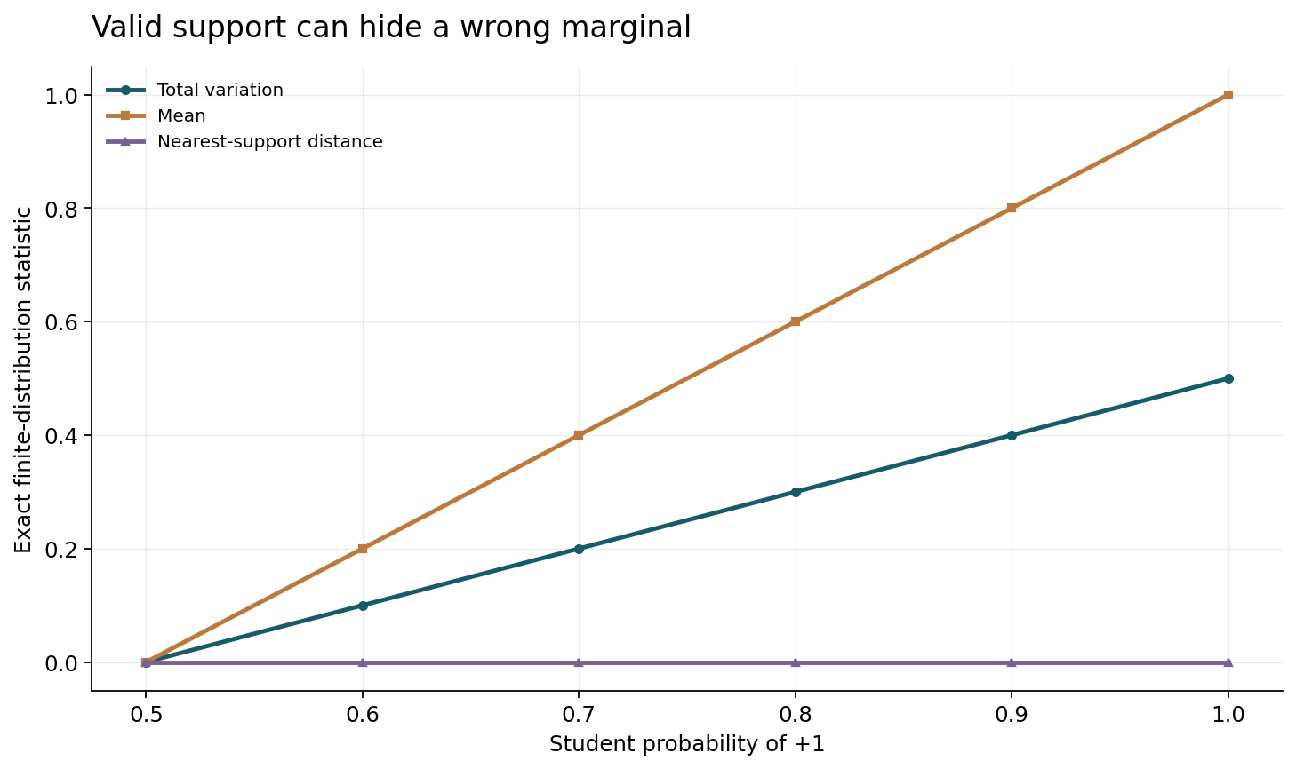
Take a target distribution placing equal probability on minus one and plus one. A student that outputs plus one with probability 0.9 and minus one with probability 0.1 always produces a value on the correct support. Any metric that checks only distance to the nearest valid support point reports zero for both target and student. Nevertheless, the total-variation distance is 0.4 and the student's mean is 0.8 instead of zero.
This finite construction isolates a distributional failure that attractive examples can hide. It does not claim that a particular image metric reduces to nearest-support distance, nor that a cited model has these probabilities. It shows why fidelity needs a declared object: individual sample validity and marginal frequency are not the same. The example can be enumerated exactly, avoiding estimation uncertainty. In an image benchmark the analogous question requires a suitable metric and enough samples, with uncertainty reporting. Rare modes and conditional subpopulations can be especially difficult to assess when results are reduced to a single average score.
5. Paired targets and distribution matching differ
A paired regression objective asks a student to resemble the teacher output associated with a particular input or noise trajectory. A distribution-level objective asks whether the aggregate outputs have the desired law. These questions can align under strong conditions, but they are not identical. A student with limited capacity can minimize a pointwise loss by smoothing distinctions that matter to the marginal distribution.
Distribution Matching Distillation explicitly addresses a distribution-level target using learned score information and an approximate objective. That makes it a useful comparator rather than simply another name for consistency training. The approximation, score estimators and auxiliary losses remain part of the method. A report should not turn the phrase distribution matching into an assertion of exact equality. The finite two-point model offers a simple audit principle: retain both correspondence errors under a fixed coupling and marginal-frequency errors. Improvement in one should not be presented as improvement in the other unless the experiment actually measures both under a justified relationship.
Sources: [6]
6. Training schedules allocate fidelity unevenly
The improved consistency-training work changes target construction, losses and noise/discretization schedules. Its relevance is that the learned map depends on where and how the training objective spends effort. A method's architecture alone does not determine the error profile across noise levels. We do not reuse its benchmark values as new measurements or assume that one schedule is best for every domain.
A training loss averaged over sampled times can be small while a narrow deployment-relevant interval remains poorly approximated. The effect depends on both the time distribution and the weighting of errors. A diagnostic should therefore report performance across noise-time strata, not only an aggregate training curve. It should also distinguish target error from model-fitting error: a student can fit a biased or coarse target accurately. When a schedule changes over training, the full schedule belongs in the reproducibility record. Comparing only the final number of discretization levels can hide substantial differences in which pairs were seen and how their gradients were weighted.
Sources: [3]
7. Latent acceleration retains a decoding boundary
Latent Consistency Models adapt few-step generation to latent diffusion pipelines and guided teachers. This moves much of the expensive iterative work into a compressed representation, but a usable image still requires a decoder and a conditioning pathway. The inspected source motivates latent endpoint prediction; it does not establish that arbitrary latent errors translate uniformly into pixel-space or semantic errors.
A decoder can be sensitive to some latent directions and insensitive to others. A latent reconstruction metric can therefore miss an output difference that matters to a user, while a visible difference may be harmless for another task. The evaluation should record the autoencoder version, latent scaling and decoding configuration with the student weights. If a compressed representation cannot preserve a requested detail, improving the sampler alone cannot recover information absent from that representation. This is a separate bottleneck from the number of denoising steps. End-to-end quality should consequently be assessed after decoding, with reconstruction limitations reported alongside sampling limitations rather than attributed entirely to the fast generator.
Sources: [4]
8. A trajectory map offers a different control surface
Consistency Trajectory Models generalize endpoint prediction to mappings between noise-time positions. That creates additional choices for deterministic or stochastic traversal and for allocating inference computation. The paper's reported improvements are evidence for its tested settings, not a theorem that every extra step improves every user-relevant quality criterion.
The interface distinction is useful. An endpoint-only map and a map that supports intermediate destinations may expose different editing or refinement operations. A comparison should state which controls are required by the application and whether they are native, approximated or unavailable. If one model supports a richer trajectory interface, giving both models the same nominal number of calls may not compare the same operation. Conversely, an application that needs only unconditional samples may not benefit from the extra interface. Evaluation should connect the sampler's control surface with concrete tasks, including how added noise, changed guidance or partial reconstruction affects consistency with user-provided conditions.
Sources: [5]
9. Guidance changes both the target and the bill
Conditional generation often combines conditional and unconditional information or otherwise changes the sampling field according to a guidance setting. The implementation may compute the branches separately or batch them together. A displayed sampling step can therefore involve a different amount of work across configurations. The output distribution can also change as guidance changes, so the comparison has both computational and statistical consequences.
A fair ledger names the guidance mechanism, scale and implementation, as well as logical model evaluations and measured latency. A teacher distilled at one guidance regime may not preserve behavior at another regime automatically. Evaluation should vary guidance only according to the intended interface contract, rather than selecting a favorable setting separately for each metric without disclosure. For text-to-image tasks, prompt adherence, sample diversity and visible artifacts may trade off differently. The goal is to expose that frontier rather than to make a one-step label carry conclusions about all guidance settings.
10. Fixed overhead limits end-to-end speedup
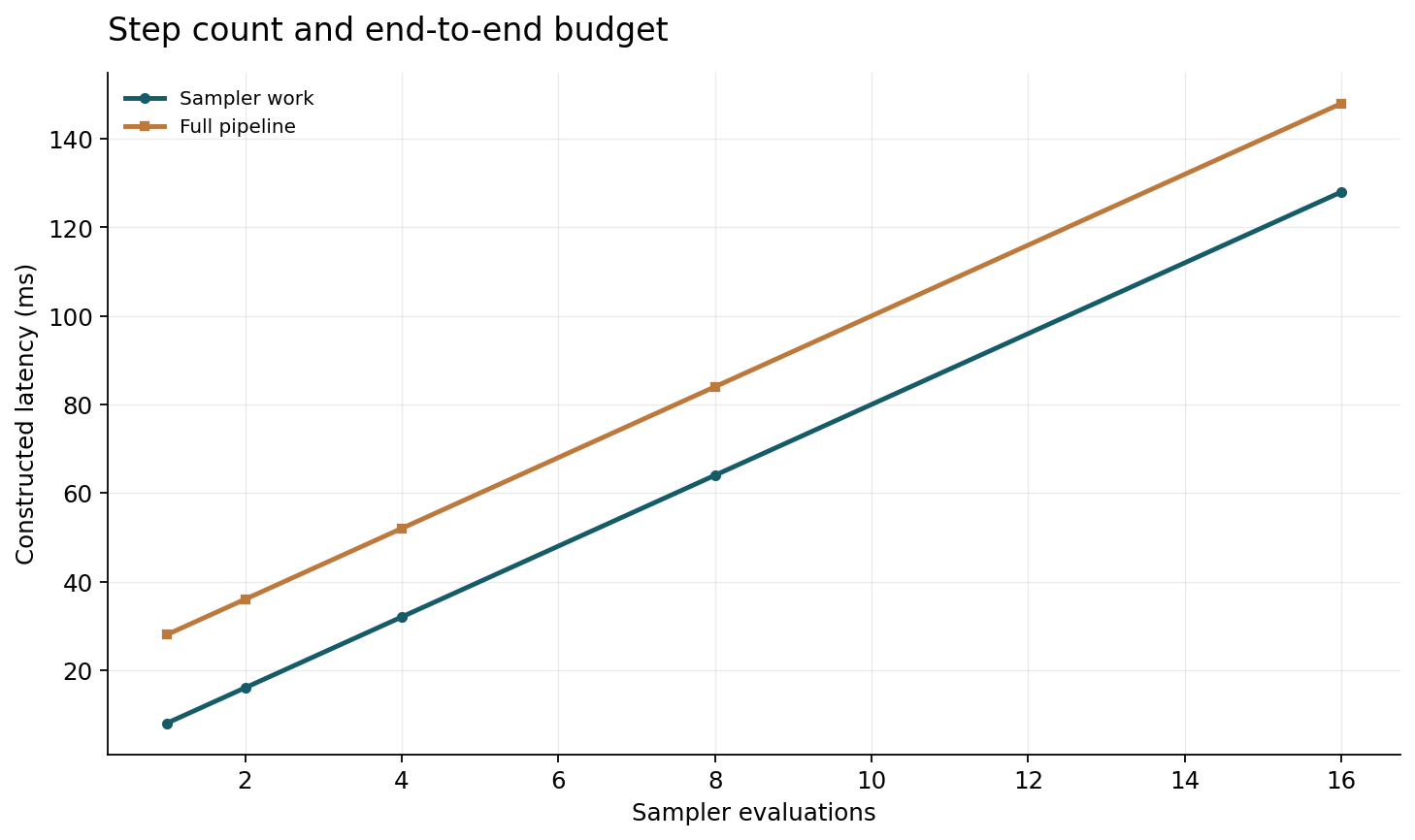
Consider a constructed pipeline with twenty milliseconds of fixed work and eight milliseconds per sampler evaluation. With sixteen evaluations, total latency is 148 milliseconds. With one evaluation, it is twenty-eight milliseconds. The sampler evaluation count falls by a factor of sixteen, while total latency improves by approximately 5.29 times. The difference follows directly from the unchanged overhead.
The numbers are assumptions for an explanatory cost model, not timings of any cited implementation or hardware. Their purpose is to force the accounting boundary into view. An actual benchmark should measure preprocessing, conditioning, sampling, decoding and postprocessing separately, then report the full user-visible latency. Batching can change each component's cost, so multiplying a single-image timing by batch size is not generally sufficient. Throughput and interactive latency should also remain separate. A fast sampler can improve both, but queueing, device utilization and fixed per-request work can affect them differently.
11. Distillation savings have an amortization horizon
Suppose the extra student-training cost is one hour and the per-image inference saving is 120 milliseconds in the constructed pipeline. Dividing the training cost by that saving gives a break-even point of thirty thousand generated images. This is an arithmetic budget comparison, not an estimate for a real training run. It assumes the teacher already exists, the student is reused unchanged and the chosen quality level is acceptable.
Those assumptions can fail. A student may need retraining for a new domain, guidance regime or output resolution. A model that saves inference cost but is replaced frequently may never reach its amortization horizon. Conversely, a widely deployed student can justify substantial training work. Reports should therefore state whether they optimize a one-off experiment, a reusable research checkpoint or a high-volume service. Including amortization does not require a speculative monetary estimate. A transparent compute ledger and deployment-volume range can show which conclusions are robust without claiming a universal economic advantage.
12. Evaluation must preserve difficult conditions
A mean quality score can improve while a subset of prompts becomes less reliable. Small text, unusual compositions, rare objects, long descriptions or domain-specific constraints may stress a compressed generator differently. Selecting appealing examples after generation does not estimate performance on the intended request distribution. A serious evaluation should fix its prompt set and sampling policy before examining outputs.
The report should retain failures, retries and discarded results in the denominator. If a fast method generates several candidates and chooses one, the selection process belongs in the compute budget and evaluation definition. If a teacher supplies an additional refinement pass for difficult cases, the service is a hybrid system and should be described as one. These practices do not require claiming that every edge case has been discovered. They prevent a systematic bias toward easy successful outputs from being mistaken for robust preservation of the teacher's capabilities at a lower step count.
13. Reproducibility requires the full target pipeline
A fast-generator artifact should identify the teacher checkpoint, student architecture, conditioning encoder, decoder, training data scope, noise schedule and objective components. It should also record the sampling schedule and guidance interface used for evaluation. Two students with identical tensor dimensions can implement different target distributions when these surrounding components differ.
The same principle applies to versioning. Updating a decoder can alter visible output even when the student is unchanged. Updating a text encoder can change the conditioning semantics. Replacing a teacher can invalidate assumptions used in distillation or evaluation. A maintenance process should re-run targeted compatibility checks after such changes and distinguish them from retraining the student. This is especially important when a checkpoint is shared across tools that silently choose default guidance or latent scaling. Reproducibility is not merely loading a file successfully; it is reconstructing the executable generator whose behavior supports the reported claim.
14. A useful quality-resource frontier is multidimensional
No single curve can fully summarize fast generation. Nominal calls, wall-clock latency, peak memory, training cost, sample fidelity, diversity and condition adherence can move differently. A useful report chooses a small set of metrics tied to its application and shows where the methods are incomparable rather than forcing every result into a global ranking.
We propose comparing methods at matched visible quality targets and at matched compute budgets, since each view answers a different question. Both comparisons should include uncertainty from sample estimation and run variation. A small improvement in a distributional metric should not be presented as decisive when its uncertainty overlaps a baseline or when the prompt distributions differ. The finite two-point example avoids estimation uncertainty only because its probabilities are stipulated exactly. Real image distributions require empirical estimators whose limitations should be stated. The framework is therefore an evaluation proposal, not an assertion that a particular existing metric captures every property of a generated image.
15. The constructed checks should resist flattering summaries
The first checker defines the two-point target and a family of students with plus-one probability ranging from one half to one. It computes total variation, means and nearest-support distance exactly. It should confirm that nearest-support distance remains zero as the distributional mismatch increases. A separate intentionally incomplete pairwise-consistency objective should accept a constant map, while an added endpoint boundary should reject that map on the missing mode. This validates the distinction without misrepresenting the cited full objectives.
The second checker computes end-to-end costs for one, two, four, eight and sixteen evaluations under the declared overhead and per-call assumptions. It checks the speedup and the thirty-thousand-image amortization calculation. Negative tests should deliberately omit fixed overhead or confuse seconds with milliseconds and fail the ledger. These illustrations do not reproduce any image model, FID result or hardware timing. They make the article's arithmetic and logical counterexamples independently inspectable.
16. A shorter sampler needs a longer specification
The selected methods reduce different parts of the generation problem: repeated numerical steps, endpoint inconsistency, latent-space traversal or distribution mismatch. Their shared interest in fast inference should not erase the differences between their targets and training signals. A method can be valuable without being equivalent to every other one-step generator, and a lower step count can be meaningful without implying the same factor of user-visible acceleration.
The practical conclusion is to specify what was preserved and what was paid. The teacher and data targets, boundary conditions, guidance, representation, decoder and deployment request distribution all belong in that specification. Our finite counterexamples show why support validity and pairwise agreement alone are insufficient, while the cost model exposes fixed overhead and amortization. Future work should make those contracts easier to compare across checkpoints and services, so that fast generation is judged by reproducible behavior under a declared budget rather than by an isolated step-count slogan.
Core equations and definitions
(1) Finite-distribution total variation; target probabilities (0.5,0.5) and student (0.1,0.9) give 0.4.
(2) An ideal consistency relation; alone it does not specify boundary behavior or marginal probabilities.
(3) Constructed cost model with fixed overhead. Not a measured generator latency.
(4) Assumes one hour of extra training, an existing teacher and 120 ms per-image savings at acceptable quality.
Constructed analytical figures
Comparison and reporting contract
| Evaluations | Constructed total ms | Speedup versus 16 calls |
|---|---|---|
| 1 | 28 | 5.285714285714286 |
| 2 | 36 | 4.111111111111111 |
| 4 | 52 | 2.8461538461538463 |
| 8 | 84 | 1.7619047619047619 |
| 16 | 148 | 1 |
Evaluation protocol
- Freeze teacher/student and all conditioning/decoding components.
- State whether the target is paired correspondence, teacher marginal or data distribution.
- Record boundary construction, noise-time sampling and objective terms.
- Count guidance branches and hybrid refinement explicitly.
- Measure full-pipeline latency and peak memory at declared batch sizes.
- Fix prompt/sample sets before inspecting outputs.
- Report failures, retries, selection and uncertainty.
- Evaluate diversity and condition adherence alongside distributional metrics.
- Include student-training and retraining costs in an amortization range.
- Version the complete executable generator rather than only student tensors.
Limitations
- Two-point examples are explanatory distributions, not image-model experiments.
- The incomplete consistency loss deliberately omits a boundary and is not the cited full objective.
- The latency and amortization numbers are stipulated assumptions.
- No published FID, speedup or training-cost result is reproduced.
- Distributional metrics do not necessarily capture every user-relevant image property.
- The six-source selection is focused rather than exhaustive.
Open research questions
- Which small compatibility tests detect when decoder or guidance changes invalidate a distilled checkpoint?
- Can fast-generator evaluation preserve rare conditional modes without requiring an impractically large generic sample set?
- How should a service choose a hybrid refinement policy while reporting its true compute and failure distribution?
Evidence and its boundaries
- Progressive distillation trains a student sampler to replace multiple deterministic teacher steps with fewer steps.
- [1] — A reduced step count does not by itself quantify full-pipeline latency or arbitrary distributional fidelity. Inspected: Primary abstract and version record describing progressive halving of a deterministic teacher sampler.
- Consistency models can map noisy states toward data endpoints and can be trained through distillation or directly.
- [2] — The complete objective and boundary construction matter; pairwise consistency alone is not the full method. Inspected: Primary abstract and bibliographic record distinguishing consistency distillation and standalone training.
- Consistency-training quality depends on target construction, loss and time sampling, not only architecture.
- [3] — Historical reported FIDs are not rerun here, and improvements need their original settings. Inspected: Primary abstract and record on teacher averaging, robust losses and noise/discretization schedules.
- Latent consistency moves the fast endpoint-prediction problem into a latent diffusion pipeline.
- [4] — Encoder/decoder and conditioning costs remain; latent fidelity does not imply exact pixel fidelity. Inspected: Primary abstract on few-step latent-space inference and distillation from guided diffusion models.
- Trajectory models generalize a single endpoint map to support traversal across noise-time intervals.
- [5] — Additional sampling flexibility is not a universal guarantee that more computation always improves every metric. Inspected: Primary abstract and version record concerning mappings between arbitrary trajectory times.
- Distribution matching explicitly targets a student's output distribution rather than only paired endpoint regression.
- [6] — Its approximate objective and learned score estimates do not constitute exact equality of arbitrary distributions. Inspected: Primary abstract and record on distribution-level matching and regression components.
References
- Progressive Distillation for Fast Sampling of Diffusion Models
Tim Salimans, Jonathan Ho. ICLR 2022 (2022). https://arxiv.org/abs/2202.00512v2Source scope
Primary abstract and version record describing progressive halving of a deterministic teacher sampler.
- Consistency Models
Yang Song, Prafulla Dhariwal, Mark Chen, Ilya Sutskever. ICML 2023 (2023). https://arxiv.org/abs/2303.01469v2Source scope
Primary abstract and bibliographic record distinguishing consistency distillation and standalone training.
- Improved Techniques for Training Consistency Models
Yang Song, Prafulla Dhariwal. arXiv preprint; ICLR 2024 paper (2023). https://arxiv.org/abs/2310.14189Source scope
Primary abstract and record on teacher averaging, robust losses and noise/discretization schedules.
- Latent Consistency Models: Synthesizing High-Resolution Images with Few-Step Inference
Simian Luo, Yiqin Tan, Longbo Huang, Jian Li, Hang Zhao. arXiv preprint (2023). https://arxiv.org/abs/2310.04378Source scope
Primary abstract on few-step latent-space inference and distillation from guided diffusion models.
- Consistency Trajectory Models: Learning Probability Flow ODE Trajectory of Diffusion
Dongjun Kim, Chieh-Hsin Lai, Wei-Hsiang Liao, Naoki Murata, Yuhta Takida, Toshimitsu Uesaka, Yutong He, Yuki Mitsufuji, Stefano Ermon. ICLR 2024 (2024). https://arxiv.org/abs/2310.02279v3Source scope
Primary abstract and version record concerning mappings between arbitrary trajectory times.
- One-step Diffusion with Distribution Matching Distillation
Tianwei Yin, Michaël Gharbi, Richard Zhang, Eli Shechtman, Fredo Durand, William T. Freeman, Taesung Park. CVPR 2024 (2024). https://arxiv.org/abs/2311.18828v4Source scope
Primary abstract and record on distribution-level matching and regression components.