
Deep Learning: Sequence Models / DEEP LEARNING III
Guidance Changes the Target: Conditional Diffusion Between Fidelity and Concentration
Guidance combines score fields to favor a condition, but the resulting field and final sampling distribution require separate interpretation.
English original. Translations of this new review are not yet available.

Abstract
Guidance combines score fields to favor a condition, but the resulting field and final sampling distribution require separate interpretation. This review derives a fixed-noise power-density identity and an exact Gaussian example showing changes in mean, variance and normalizability. It distinguishes conditional fidelity, diversity, numerical error and cross-time consistency, then proposes controlled evaluation of guidance schedules. The curves are analytical constructions and do not represent image-generation benchmark measurements.
In this paper
- 1. A stronger condition is a different objective
- 2. What the primary records establish
- 3. Fix a convention before discussing scale
- 4. The fixed-noise power-density identity
- 5. An exact Gaussian calculation
- 6. Concentration and fidelity are not synonyms
- 7. Normalizability is an assumption
- 8. Exact local scores do not ensure temporal consistency
- 9. Learned score errors are also amplified
- 10. Numerical solvers add another approximation
- 11. Guidance schedules should be evaluated as policies
- 12. Conditional quality needs multiple measurements
- 13. A controlled research protocol
- 14. What the executable checks establish
- 15. Interpreting guidance improvements
- 16. Open questions and limitations
1. A stronger condition is a different objective
Conditional generation asks for samples compatible with a condition, but compatibility can be interpreted in several ways. A model may represent the full conditional distribution, concentrate on its most recognizable modes, or optimize a separate score that rewards visible alignment. Increasing guidance can improve one of these properties while changing another.
The central issue is therefore the sampling target. A guidance rule combines learned vector fields, and that combination may correspond locally to a reweighted density under ideal assumptions. It does not automatically follow that a finite-step sampler produces the desired final distribution. This review separates the fixed-noise algebra from the time-dependent process and from numerical implementation. A Gaussian construction gives exact means and variances for a power-reweighted density. A second control identifies parameter regimes where the proposed density is not normalizable. These examples are intentionally simple. They clarify the assumptions behind guidance language without claiming that a real image model is Gaussian or that a local identity proves the correctness of a complete diffusion sampler.
2. What the primary records establish
Dhariwal and Nichol study classifier guidance for conditional image synthesis. Ho and Salimans introduce classifier-free guidance by combining conditional and unconditional estimates. The DDPM work develops denoising diffusion probabilistic modeling, while the score-SDE work formulates time-dependent score-based generation. DDIM studies alternative sampling processes compatible with diffusion training objectives.
Imagen studies text-conditioned diffusion generation and reports architectural and evaluation choices for that setting. Together, these sources motivate distinguishing training, conditioning and sampling. Our review uses the inspected original abstracts and bibliographic records for these broad methodological roles. It does not reproduce their image benchmarks, verify complete proofs or claim that historical quality rankings remain current. The analytical developments below are authored controls. They use exact scores of declared densities to examine what a guidance combination means at one noise level. That limited setting allows the algebra to be checked cleanly, while leaving the behavior of learned, approximate, time-dependent neural samplers as a separate empirical and theoretical question.
3. Fix a convention before discussing scale
Let s_u be an unconditional score and s_c a conditional score at the same noise level. Define guided score s_g=s_u+g(s_c-s_u). Under this convention, g=0 is unconditional and g=1 is the ordinary conditional score. Values above one extrapolate beyond the conditional score in the difference direction.
Other software and papers may use a parameter whose zero corresponds to ordinary conditional sampling. Comparing numerical guidance values without translating conventions can therefore be meaningless. The implementation should state the exact formula, the parameterization of the model output and any rescaling applied afterward. Noise prediction, clean-sample prediction and score prediction are related through schedule-dependent factors, so an apparently identical linear combination can be implemented at different stages. A reproducible experiment records those details alongside the schedule. The Gaussian examples here use the score convention directly, with exact analytical densities. They do not assume that every package's guidance-scale argument has the same interpretation or that a value used in one model transfers unchanged to another.
4. The fixed-noise power-density identity
Assume positive differentiable densities p_u and p_c at one fixed noise level, with exact scores equal to gradients of their log densities. The guided field is then the gradient of the logarithm of p_c raised to g times p_u raised to one minus g. If this product is integrable, it can be normalized into a density q_g.
The identity is local in noise level and depends on exact conservative score fields. It does not by itself establish that the sequence of q_g densities across noise levels is the forward-noising family of some endpoint distribution. Nor does it establish that a numerical reverse process using those fields samples q_g at the final time. These are stronger consistency questions. The distinction is often lost when the power-density expression is presented as the final sampling law without qualification. In this review, the expression is used only as a fixed-noise diagnostic. It reveals how extrapolating a conditional score can change concentration and location, and it provides a tractable example where normalizability can be checked explicitly.
5. An exact Gaussian calculation
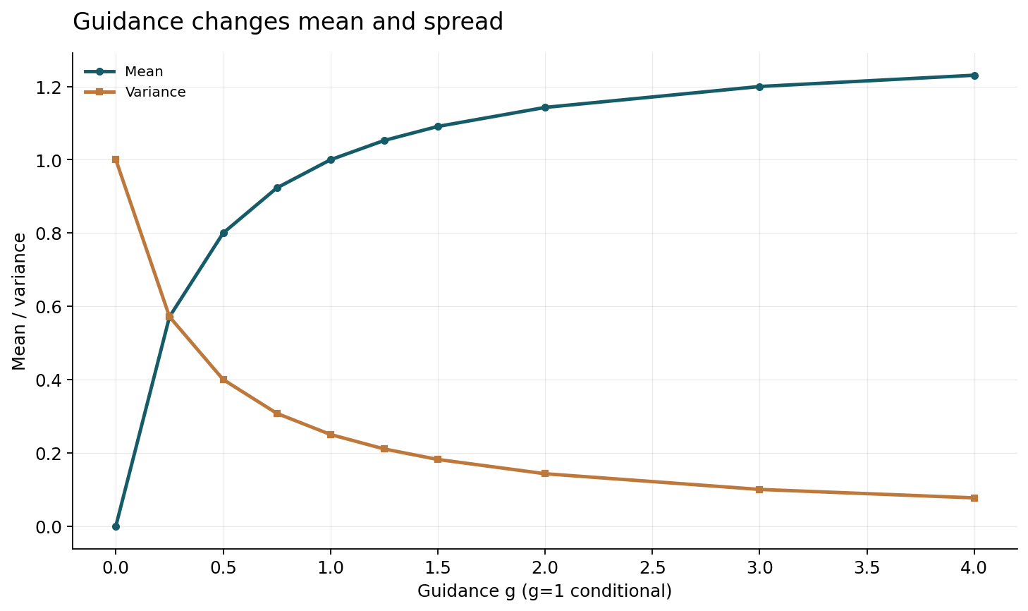
Let the unconditional density be a one-dimensional normal distribution with mean zero and variance one. Let the conditional density have mean mu and variance sigma_c squared. The power product has quadratic precision tau_g=g/sigma_c squared plus one minus g. When tau_g is positive, the normalized product is Gaussian with variance one divided by tau_g and mean equal to g mu divided by sigma_c squared times tau_g.
This formula follows by collecting the quadratic and linear terms in the exponent and completing the square. Figure one uses mu=1 and sigma_c squared equal to one quarter. Under these choices, precision is one plus three g, variance decreases as guidance grows, and the mean approaches four thirds rather than remaining fixed at the conditional mean one. At g=1 the ordinary conditional density is recovered exactly. This construction shows that extrapolated guidance can alter both concentration and location. It is not a claim that image-space means behave in the same way, but it refutes an interpretation in which guidance merely samples the original conditional distribution more accurately without changing the target.
6. Concentration and fidelity are not synonyms
In the Gaussian example, reducing variance makes samples more concentrated, but concentration alone does not establish better fidelity to the ordinary conditional distribution. At g greater than one, both the variance and mean differ from that distribution. A metric rewarding proximity to a preferred region may improve while distributional coverage declines.
The appropriate evaluation depends on the goal. If the user wants a prototypical sample, concentration may be desirable. If the task requires calibrated uncertainty or coverage of plausible alternatives, the same concentration may be harmful. A report should therefore distinguish condition alignment, perceptual quality, diversity and distributional fidelity. No single scalar automatically captures all four. The Gaussian control makes this distinction visible because the full distribution is known. In real models, one must approximate these properties through suitable metrics and human or task-specific evaluation. Those measurements should not be interpreted as proof that the guided sampler matches the original data conditional unless that is actually what the evaluation tests.
7. Normalizability is an assumption
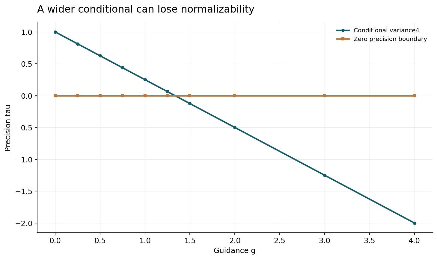
Choose instead a conditional variance greater than the unconditional variance. Then the guided precision can decrease as g increases. For example, with conditional variance four, tau_g equals one minus three quarters g, which reaches zero at g equal to four thirds. Beyond that point, the power product grows in the tails and cannot be normalized over the real line.
Figure two plots the precision and its zero boundary explicitly; the variance is defined only where precision is positive. It does not assign a finite variance to the non-normalizable regime. This is a fixed-noise counterexample to assuming that every extrapolated score combination defines a probability density. Actual neural diffusion systems may operate under distributions and schedules where this specific pathology does not occur, and finite numerical domains can obscure tail behavior. The point is logical: integrability must be justified, not inferred from the fact that the two original densities were valid. Negative powers of a density can amplify regions where that density is small. Extrapolation above g=1 introduces precisely that possibility in the chosen convention.
8. Exact local scores do not ensure temporal consistency
A diffusion sampler uses scores at many noise levels, not just one. Even if each guided field is the score of a normalizable density q_g,t, the family of these densities may not evolve under the same forward-noising process assumed by the reverse dynamics. A collection of individually valid marginals is not automatically a consistent stochastic process.
This distinction is especially important when the guidance strength changes with time. A schedule can be a useful heuristic or an empirically successful design, but its interpretation requires more than the fixed-time power formula. One should ask whether the schedule corresponds to a known target, an approximate correction or a deliberate change in sampling behavior. The present review does not prove a general impossibility or a general consistency theorem. It identifies the missing step in a common argument: deriving a local score identity does not complete the derivation of the endpoint distribution. Exact small distributions and numerically solved low-dimensional processes can help test that step before drawing conclusions from high-dimensional sample quality alone.
9. Learned score errors are also amplified
Suppose the estimated conditional and unconditional scores contain errors e_c and e_u. The guided error under the declared convention is g e_c+(1-g)e_u. For large g, even modest errors can be magnified, depending on their correlation and direction. If the two errors cancel, guidance may reduce some components; if they reinforce, it may increase them.
A bound based on norms gives at most g times the conditional error norm plus the absolute value of one minus g times the unconditional error norm. This is conservative and does not determine actual sample quality. It does, however, show why guidance strength interacts with estimator accuracy. An experiment should compare error-sensitive behavior across noise levels rather than treating the guidance coefficient as a purely semantic control. Approximate scores may also fail to be exact gradients of any density, further limiting the power-density interpretation. These issues are separate from discretization error in the sampler. Measuring one while ignoring the other can misattribute artifacts or instability to the wrong component.
10. Numerical solvers add another approximation
A finite-step sampler approximates a continuous or discrete generative process using a particular schedule and update rule. Increasing guidance can change the magnitude and curvature of the vector field, potentially making the same step schedule less accurate. A comparison that changes guidance while holding a coarse solver fixed therefore mixes target change with numerical approximation.
A useful control repeats the experiment at increasing step resolution and compares several solver settings under matched evaluation budgets. Convergence on a low-dimensional distribution with known reference behavior can reveal implementation errors before image-generation metrics are used. Wall-clock cost should be reported because additional score evaluations can change the practical tradeoff. Deterministic and stochastic samplers also require different uncertainty accounting. The present Gaussian fixed-noise figures are not solver trajectories, and their captions state that limitation. They provide exact reference densities for local reasoning. Any claim about the complete sampler must be supported by a separate integration experiment that specifies the time parameterization, initial distribution, noise schedule and numerical tolerances.
11. Guidance schedules should be evaluated as policies
A time-varying guidance schedule allocates condition pressure across noise levels. It may emphasize broad structure early, details later or another empirically useful pattern. Such interpretations are hypotheses about the model's representation and dynamics, not consequences of the schedule alone.
An evaluation should compare schedules with a fixed model and clearly defined compute budget. If schedules are selected using the final test set, apparent gains may reflect tuning rather than generalization. Report the search space, validation criterion and sensitivity to nearby settings. Include cases where guidance harms the task, such as prompts requiring diverse plausible outcomes or rare modes. A single visually appealing sample is insufficient evidence because random seed selection can dominate the impression. The relevant unit is a distribution of outputs under declared conditions. For scientific uses, the schedule may also affect uncertainty calibration, which cannot be judged by aesthetics. A policy that improves prompt adherence can still distort the distribution needed for downstream inference.
12. Conditional quality needs multiple measurements
A rigorous evaluation separates whether samples satisfy the condition, resemble the intended data domain, cover plausible variation and avoid unsupported artifacts. These properties can conflict. A metric based on a learned embedding may reward certain recognizable features while missing subtle compositional errors or diversity loss.
Use multiple independent measurements and inspect disagreements rather than averaging them immediately. Human evaluation should specify the question asked of raters and whether they compare typicality, realism, condition adherence or preference. Automated metrics should be validated for the relevant domain. If the application requires a distribution, evaluate coverage and calibration in addition to sample quality. For a deterministic illustration task, a different utility may be appropriate. The Gaussian control underscores why the objective must be explicit: higher concentration can be good for one purpose and wrong for another. None of the source benchmark numbers is reproduced here, and the review does not claim that its analytical variance curves predict perceptual scores in image generation.
13. A controlled research protocol
Start with exact low-dimensional conditional and unconditional distributions. Verify the score convention, the fixed-time power identity and the region of normalizability. Then run the intended sampler with increasingly fine schedules and compare its endpoint distribution with an appropriate numerical reference. This separates algebraic target questions from solver errors.
For learned models, freeze the model and evaluation prompts while varying guidance and schedule. Report all selected seeds, compute cost, condition alignment and diversity metrics. Include ablations for score rescaling, clipping or thresholding because they change the field beyond the simple linear combination. Keep validation and final evaluation separate. Publish failure cases and sensitivity curves rather than only the best setting. The protocol is proposed, not executed at neural scale in this review. The finite companion program verifies the exact constructions used in the figures, providing a small but useful foundation for the broader experiment. A strong empirical result would then state which objective improved and what distributional or numerical costs accompanied that improvement.
14. What the executable checks establish
The program computes Gaussian precision, mean and variance for the declared parameter sets. It verifies recovery of the unconditional density at g=0 and the conditional density at g=1. It compares the derivative of the completed-square log density with the guided combination of the original Gaussian scores at several points.
For the wider conditional distribution, it checks the exact positivity boundary and refuses to report a variance when precision is nonpositive. Figure data in the valid region are generated from the same formulas; the invalid region is represented by precision values rather than fabricated finite variances. These checks validate the algebra and the illustrations. They do not train a diffusion model, simulate a complete reverse process or reproduce source image-quality results. That scope is intentional. A mathematically correct local example can reveal a hidden assumption without being promoted into a universal description of high-dimensional neural sampling. Readers can change the parameters and observe how normalizability and concentration depend on the stated density family.
15. Interpreting guidance improvements
A useful claim says that a particular guidance policy improves a specified metric on a specified distribution under a specified sampling budget. It should not automatically be restated as more accurate conditional sampling. If the policy intentionally concentrates on preferred modes, that is a change in objective rather than merely a reduction in approximation error.
The distinction supports better engineering decisions. A creative image system may favor recognizable condition adherence, while a scientific uncertainty model may require calibrated variation. The same guidance value can be appropriate in one and misleading in the other. Evaluation should follow the intended use. The exact Gaussian example demonstrates why location and spread can both change, and the non-normalizable example shows why even a local density interpretation needs assumptions. These are not arguments against guidance. They are arguments for describing what it does precisely. A successful method can be celebrated for its actual benefits without attaching an unsupported claim that it preserves the original conditional distribution in every regime.
16. Open questions and limitations
Important questions remain about when guided score families are temporally consistent, how learned-score error interacts with strong conditioning, and which schedules offer reliable tradeoffs across domains. Low-dimensional reference problems can support theory and debugging, while high-dimensional experiments are needed to establish practical quality and robustness.
This review contributes no new image benchmark or neural training result. Its original work is a set of exact local calculations and executable checks, combined with a focused primary-source overview. The conclusions are correspondingly bounded: guidance conventions must be explicit, extrapolation can change the local target, integrability is not automatic, and endpoint claims require more than a fixed-time identity. These distinctions make future studies easier to interpret and reproduce. They also give practitioners a concrete way to reason about a familiar control whose numerical simplicity can conceal substantial changes in the distribution being generated.
Core equations and definitions
(1) Convention: g=0 unconditional, g=1 ordinary conditional.
(2) Fixed-noise identity only, when exact scores and a finite normalizer exist.
(3) Precision for p_u=N(0,1), p_c=N(mu,sigma_c squared).
(4) Mean and variance of the normalized Gaussian power product.
(5) Exact algebraic combination of conditional and unconditional score errors.
Constructed analytical figures
Comparison and reporting contract
| Object | What it establishes | What it does not establish |
|---|---|---|
| Fixed-time score identity | A local power-product gradient | Correct endpoint sampling |
| Concentration | Reduced spread under a declared density | Faithful conditional coverage |
| Improved sample metric | Better measured objective | Universal distributional correctness |
Evaluation protocol
- State the guidance formula and output parameterization.
- Check exact low-dimensional targets before neural experiments.
- Separate schedule convergence from target changes.
- Report condition adherence, coverage and cost independently.
Limitations
- Only fixed-noise Gaussian constructions are computed.
- No complete reverse process is simulated.
- No neural image benchmark or source experiment is reproduced.
Open research questions
- When are guided marginal families consistent with a diffusion process?
- How do score-error correlations affect strong guidance?
- Which schedule evaluations preserve uncertainty requirements?
Evidence and its boundaries
- Studies classifier guidance for conditional synthesis.
- [1] — Original arXiv bibliographic record and abstract inspected on 2026-10-28; full proof and source experiments not independently audited. Inspected: Primary arXiv abstract and bibliographic record.
- Introduces conditional/unconditional score combination without a separate classifier.
- [2] — Original arXiv bibliographic record and abstract inspected on 2026-10-28; full proof and source experiments not independently audited. Inspected: Primary arXiv abstract and bibliographic record.
- Develops denoising diffusion probabilistic modeling.
- [3] — Original arXiv bibliographic record and abstract inspected on 2026-10-28; full proof and source experiments not independently audited. Inspected: Primary arXiv abstract and bibliographic record.
- Formulates time-dependent score-based generation through SDEs.
- [4] — Original arXiv bibliographic record and abstract inspected on 2026-10-28; full proof and source experiments not independently audited. Inspected: Primary arXiv abstract and bibliographic record.
- Studies alternative sampling processes compatible with diffusion training.
- [5] — Original arXiv bibliographic record and abstract inspected on 2026-10-28; full proof and source experiments not independently audited. Inspected: Primary arXiv abstract and bibliographic record.
- Studies text-conditioned diffusion image generation.
- [6] — Original arXiv bibliographic record and abstract inspected on 2026-10-28; full proof and source experiments not independently audited. Inspected: Primary arXiv abstract and bibliographic record.
References
- Diffusion Models Beat GANs on Image Synthesis
Prafulla Dhariwal, Alex Nichol. arXiv primary author manuscript (2021). https://arxiv.org/abs/2105.05233Source scope
Original arXiv bibliographic record and abstract inspected on 2026-10-28; full proof and source experiments not independently audited.
- Classifier-Free Diffusion Guidance
Jonathan Ho, Tim Salimans. arXiv primary author manuscript (2022). https://arxiv.org/abs/2207.12598Source scope
Original arXiv bibliographic record and abstract inspected on 2026-10-28; full proof and source experiments not independently audited.
- Denoising Diffusion Probabilistic Models
Jonathan Ho, Ajay Jain, Pieter Abbeel. arXiv primary author manuscript (2020). https://arxiv.org/abs/2006.11239Source scope
Original arXiv bibliographic record and abstract inspected on 2026-10-28; full proof and source experiments not independently audited.
- Score-Based Generative Modeling through Stochastic Differential Equations
Yang Song, Jascha Sohl-Dickstein, Diederik P. Kingma, Abhishek Kumar, Stefano Ermon, Ben Poole. arXiv primary author manuscript (2020). https://arxiv.org/abs/2011.13456Source scope
Original arXiv bibliographic record and abstract inspected on 2026-10-28; full proof and source experiments not independently audited.
- Denoising Diffusion Implicit Models
Jiaming Song, Chenlin Meng, Stefano Ermon. arXiv primary author manuscript (2020). https://arxiv.org/abs/2010.02502Source scope
Original arXiv bibliographic record and abstract inspected on 2026-10-28; full proof and source experiments not independently audited.
- Photorealistic Text-to-Image Diffusion Models with Deep Language Understanding
Chitwan Saharia, William Chan, Saurabh Saxena, Lala Li, Jay Whang, Emily Denton, Seyed Kamyar Seyed Ghasemipour, Burcu Karagol Ayan, S. Sara Mahdavi, Rapha Gontijo Lopes, Tim Salimans, Jonathan Ho, David J Fleet, Mohammad Norouzi. arXiv primary author manuscript (2022). https://arxiv.org/abs/2205.11487Source scope
Original arXiv bibliographic record and abstract inspected on 2026-10-28; full proof and source experiments not independently audited.