

Abstract: Map Detail and the Precision of Evidence
Forest carbon maps can display continuous, detailed spatial textures, but those textures do not directly indicate that each location has been measured independently. Drawing on GEDI footprint biomass models and research on cross-scale inference, this article examines the evidence chain from laser returns and plot calibration to regional totals. We distinguish prediction maps, design-supported means, and changes between periods, explaining why increasing the number of pixels cannot eliminate shared calibration bias and how to maintain a complete uncertainty ledger.[1] Aboveground biomass density models for NASA’s Global Ec[2] GEDI launches a new era of biomass inference from space
English abstract
Spaceborne lidar connects canopy structure to biomass through calibration and statistical sampling. We examine footprint-to-region inference, nested error and forest-type representation, and derive variance and stratification examples. The analysis distinguishes fine-resolution maps from independently supported carbon stock and stock-change estimates.
The Modeling Layer from Waveforms to Biomass
Duncanson and colleagues present GEDI footprint-scale biomass models, using ground and airborne lidar-related data to establish links between waveform height metrics and biomass. This demonstrates a calibration relationship between structural observations and biomass inference, rather than enabling lasers to weigh carbon directly. Models are differentiated by vegetation and geographic context, indicating that the same height signal cannot unconditionally correspond to a uniform biomass value. This article does not recast footprint-model performance figures as guarantees for any forest worldwide.[1] Aboveground biomass density models for NASA’s Global Ec
Contributions of a Cross-Scale Statistical Framework
Dubayah and colleagues use GEDI observations to provide biomass estimates and standard errors at different scales, emphasizing the integration of sampling and statistical inference. For regional totals, the spatial coverage and weighting of observations are as important as point-level model error. This article treats that study as a case of design-supported inference, neither equating the number of grid predictions with the number of independent samples nor automatically treating aboveground biomass as total ecosystem carbon.[2] GEDI launches a new era of biomass inference from space
The Observational Target Must First Be Defined
Aboveground woody biomass, belowground roots, litter, and soil carbon belong to different pools. Converting tree height to aboveground biomass and then multiplying by a carbon fraction still does not directly measure the other carbon pools. Every conversion requires units, scope, and assumptions. If a report uses the umbrella term “forest carbon,” it should specify which components are included; otherwise, different studies may be comparing entirely different stocks that are mistakenly considered directly additive because they share the same units.作者分析与复核建议 / Author analysis
Spatial Mismatch Between Footprints and Plots
Even when a laser footprint and a ground plot have nearby centers, their boundaries, positioning errors, and canopy occlusion may differ. In heterogeneous forests, small misalignments can produce substantial differences. Calibration should document plot area, measurement date, and spatial registration, rather than assigning every discrepancy to model residuals. If ground measurements and remote sensing span a disturbance or a period of growth, temporal mismatch also becomes a source of systematic error.作者分析与复核建议 / Author analysis
Upstream Uncertainty in Allometric Relationships
Ground-based biomass is often estimated from tree diameter, height, wood density, and allometric models; it is not error-free ground truth. Remote sensing models fitted to these estimates inherit their biases. In particular, when an allometric equation is unsuitable for a forest type, more remote sensing footprints cannot automatically correct it. Research should track ground-model versions and input errors, and distinguish shared calibration uncertainty from independent measurement noise in regional inference.作者分析与复核建议 / Author analysis
How Stratification Weights Change the Mean
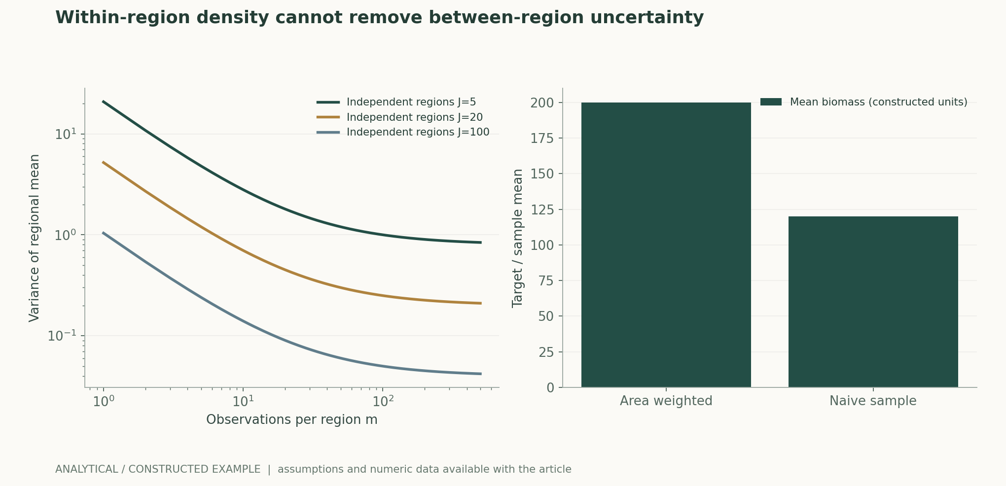
Consider two constructed forest types with biomass densities of 100 and 300, each occupying half the actual area, giving a population mean of 200. If the high-biomass type accounts for only 10% of the sample, the simple sample mean is just 120. This difference concerns representativeness and weighting, not sensor performance. The figure varies the areas of the two types and the sample composition, illustrating that more samples may estimate a skewed sample mean more precisely rather than the mean of the target region.作者分析与复核建议 / Author analysis
Spatial Correlation Reduces Additional Information
Adjacent footprints may share forest type, terrain, and calibration errors, and cannot simply be regarded as independent. Dividing a large homogeneous forest into more pixels only changes the resolution of its representation and does not necessarily add independent information. This article uses a nested variance model to distinguish between-region variation from within-region noise; increasing measurements in each region can reduce the latter, whereas the former requires more independent regions. This model is a sampling counterexample, not a fit to actual GEDI errors.作者分析与复核建议 / Author analysis
Spatial Separation of Training and Validation
Randomly splitting footprints may place neighbors from the same stand in both training and test sets, making a model appear capable of predicting distant forests. More appropriate tests of extrapolation should hold out spatial blocks, forest types, geographic regions, or time periods. Different splits answer different questions and need to be identified explicitly. If deployment targets include high biomass or complex terrain absent from training, the model should flag extrapolation and provide wider uncertainty rather than reuse the average in-domain error.作者分析与复核建议 / Author analysis
Model Saturation and Tail Bias
When observational metrics become insensitive to changes at high biomass levels, predictions tend to shrink toward the training mean. Overall error may be modest, yet high-stock areas may be systematically underestimated and low-stock areas overestimated. Conditional residuals and tail strata should be examined, rather than reporting only a single global correlation coefficient. The sensitivity of regional totals to these biases also depends on the area of each forest type, so rankings of point-level errors do not necessarily correspond to rankings of total errors.作者分析与复核建议 / Author analysis
Carbon Change Is Not Simply the Difference Between Two Maps
Errors in estimates from two periods may be correlated. The variance of change requires the variances for both periods and their covariance; error bars cannot mechanically be added as if independent, nor can complete cancellation be assumed simply because the same model is used. If the reference model is updated between periods, methodological changes are also mixed in. Credible change detection should keep definitions fixed where possible, compare common coverage, and specify how growth, harvesting, fires, and missing data enter temporal alignment.作者分析与复核建议 / Author analysis
Locations with Missing Data May Be Particularly Important
Clouds, terrain, sensor-quality filtering, or orbital sampling may make some areas less likely to enter the set of valid observations. If missingness is related to forest type, disturbance, or biomass, simply imputing surrounding averages may introduce bias. Research should disclose quality rules and effective-coverage maps, and compare totals under different missingness models. Attractive continuous map layers must not conceal locations that lack direct support, and imputed values in particular must not be labeled as observations.作者分析与复核建议 / Author analysis
Area Boundaries and Classification Error
Definitions of forest extent, land cover, and management boundaries change area weights. Even if a pixel’s biomass estimate is correct, misclassification of whether it belongs to the target forest can still shift the regional total. Classification error should be distinguished from density error, and sensitivity should be examined near boundaries. Aggregation across administrative regions especially requires a fixed boundary version; otherwise, part of the change in totals may result from updated map definitions.作者分析与复核建议 / Author analysis
Uses of Uncertainty Intervals
Intervals should refer to a clearly defined target: a single-footprint prediction, a regional mean, a regional total, or a change between periods. Their components and widths differ. A narrow interval does not imply the absence of model-specification error; actual coverage should be checked using independent regions and batches. If high-confidence conclusions are released simultaneously for many small areas, multiple comparisons and spatial dependence must also be considered. Displaying a uniform type of error bar can mislead readers about the strength of evidence for each product.作者分析与复核建议 / Author analysis
AI Fusion Models Should Preserve Links to Original Measurements
Combining lidar, optical, and radar data can expand spatial coverage, but the resulting fine pixels should retain traceability to the original footprints and calibration samples. Research needs to document each sensor’s dates, input quality, and contribution, and evaluate performance in entirely unseen regions. A model that mainly learns geographic location and forest-type priors may also produce attractive textures; sensor ablation and cross-period tests should confirm that additional information comes from genuine structural observations.作者分析与复核建议 / Author analysis
How Analytical Models Inform Design
The nested variance equation can compare the benefits of “denser sampling within the same region” and “adding independent regions”; the stratified-mean example can reveal omitted area weights. All parameters are constructed values and do not refer to actual forest stocks. Independent recalculation should recover the same results through direct enumeration and covariance operations. Such models help identify design blind spots but cannot replace actual orbital sampling, allometric calibration, or a global error budget.作者分析与复核建议 / Author analysis
Falsifiable Optimization Objectives
An improved model should reduce bias in regional means in regions held out in advance, while remaining calibrated in the high-stock tail and in analyses of sensitivity to missingness. If it only improves correlation under random pixel splits while worsening regional totals, this does not support its intended use. The primary endpoints for map display, stock estimation, and change detection should be specified in advance, avoiding the use of metrics favorable to one objective to substitute for failures on others.作者分析与复核建议 / Author analysis
Research Package and Conclusions
Materials for verification should include footprints, times, plots and allometric-model versions, spatial splits, area weights, quality filtering, and error propagation. Where original data are restricted by licenses, sufficient lawful summaries and computational procedures should still be provided. Reliable forest carbon monitoring comes from making scaling steps inspectable and keeping missingness and shared biases visible. Genuine progress is a verifiable reduction in regional inference error, rather than merely smaller map grids and smoother colors.作者分析与复核建议 / Author analysis
Core Equations and Derivations
(1) Area weights are not the same as sample proportions.
LaTeX
\bar B=\sum_h w_h\bar B_h,\quad \sum_h w_h=1(2) A simplified nested model with J independent regions and m observations in each.
LaTeX
\operatorname{Var}(\bar Y)=\tau^2/J+\sigma^2/(Jm)(3) Differences between periods require covariance.
LaTeX
\operatorname{Var}(B_2-B_1)=v_1+v_2-2\operatorname{Cov}(B_1,B_2)(4) Conversion to aboveground carbon requires area, density, and carbon fraction, and excludes other pools.
LaTeX
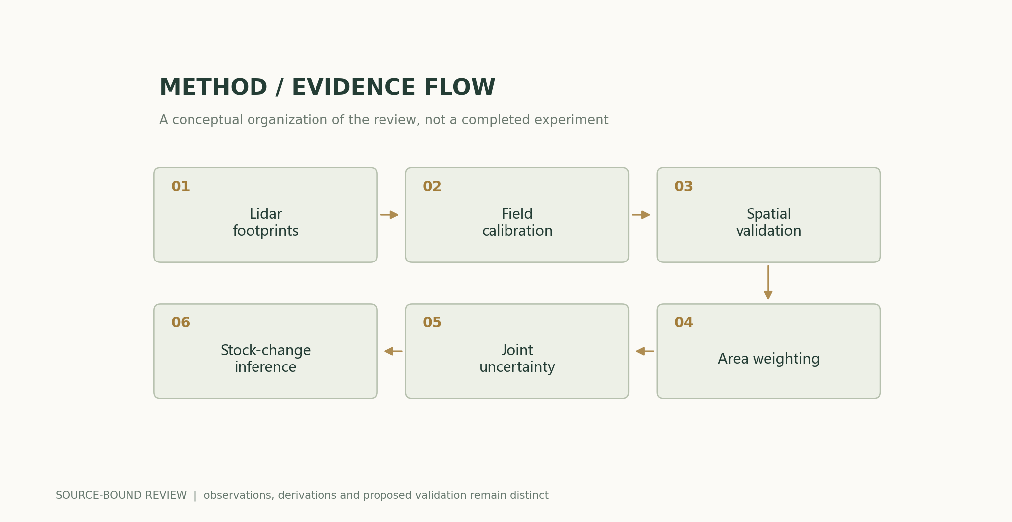
C_{\rm above}=\sum_h A_h\bar B_h f_{C,h}Methods and Evidence Workflow
Analytical Figures and Numerical Examples
Reproducible Worked Example
For two forest types with values of 100 and 300 and equal areas, the population mean is 200; when 90% of the sample comes from the lower-value type, the naive mean is 120. At J=20, the variance is 0.2+5/m; increasing m cannot eliminate 0.2.
Comparison of Methods
| Method or definition | Direct constraint | Evidence still needed |
|---|---|---|
| Waveform height | Canopy structure | Wood density and allometric conversion |
| Footprint prediction | Local model output | Calibration error and spatial matching |
| Fine-pixel fusion map | Continuous spatial representation | Additional independent observations |
| Stratified regional mean | Target-region statistic | Area and missingness mechanism |
| Difference between periods | Stock change | Covariance and model versions |
| Total ecosystem carbon | Total across multiple pools | Measurements of roots, soil, and other carbon pools |
Verification and Experimental Plan
- Fix the carbon pools, units, and target-region boundaries.
- Preserve spatiotemporal matching of footprints and plots.
- Record allometric equations and ground-calibration errors.
- Hold out regions and forest types for independent validation.
- Weight by target area rather than sample proportions.
- Propagate spatial correlation and shared model errors.
- Check cross-period covariance and sensitivity to missingness.
- Publish maps, effective coverage, weights, and exact version information.
Scope and Limitations
- There are no new lidar, plot, or carbon-stock measurements.
- Constructed variance parameters do not represent actual GEDI performance.
- Aboveground biomass is not all ecosystem carbon.
- Pixel counts cannot guarantee spatial representativeness.
- Model changes between periods cannot be treated as real stock changes.
Evidence from the Original Studies and Its Scope
| Original study results | Scope | Source and location |
|---|---|---|
| Footprint biomass models depend on waveform metrics and stratified calibration. | The scope of the original calibration data and models. | Aboveground biomass density models for NASA’s Global Ecosystem Dynamics Investigation (GEDI) lidar missionAbstract; calibration and selection |
| The GEDI inference framework supports means and standard errors at different scales. | Actual sampling design and statistical assumptions. | GEDI launches a new era of biomass inference from spaceAbstract; inference framework |
Research Questions Worth Testing
- Which is more effective: denser sampling within regions or adding independent regions?
- How do errors in the high-stock tail affect the total?
- When can shared biases cancel across periods?
Primary Sources and Corresponding Claims
- Aboveground biomass density models for NASA’s Global Ecosystem Dynamics Investigation (GEDI) lidar missionLaura Duncanson, James R. Kellner, John Armston, Ralph Dubayah, David M. Minor, Steven Hancock, et al. · 2022-03Abstract; calibration and model selection
- GEDI launches a new era of biomass inference from spaceRalph Dubayah, John Armston, Sean P Healey, Jamis M Bruening, Paul L Patterson, James R Kellner, et al. · 2022-08-18Abstract; statistical inference framework
Citation and Article Export
BibTeXRISCSL JSONTXTArticle JSON
Author, Version, and Sources
A sourced research review and original analysis written by Codex (AI). Experiments in the original papers belong to the original research teams; calculations in this article test only the listed equations and explicit assumptions. This site does not yet have records of independent peer review or original model, clinical, or physical experiments for this article.
First publication: an in-depth interdisciplinary feature on scientific evidence; retaining section-by-section sources and the boundaries between evidence from original studies and the author’s analysis.
The conceptual cover was generated by ImageGen. Scientific figures were produced using the accompanying code and numerical files, with captions specifying assumptions and measurement definitions individually.
Sources of the Cover and Scientific Figures · Data, Sources, and Assumptions · Python · Reproducible code · Publication and Version History
Source revision: 500575872cce7c4b9c4062a12bb0692eb580c2da