

Abstract
Climate simulation requires not only agreement with observations over a few days, but also reasonable long-term statistics, energy and moisture budgets, and responses to external forcing. NeuralGCM connects a differentiable large-scale dynamical core with learned parameterizations, offering a hybrid approach to unifying weather and climate tasks. This article examines which constraints this architecture can retain and which still require independent validation. Through a scalar recurrence and an energy-balance model, we show that short-term prediction error, long-term stability, and equilibrium sensitivity are not equivalent. All parameters in the figures are explicitly specified; they are neither climate forecasts from this site nor estimates of future warming.[1] Neural general circulation models for weather and clima[2] WeatherBench 2: A benchmark for the next generation of
English abstract
Hybrid atmospheric models combine explicit dynamics with learned unresolved physics. We examine NeuralGCM through a stability-and-forcing framework, distinguishing short-range skill, long-run statistics and response to new boundary conditions. A scalar recurrence demonstrates that low one-step error does not ensure stable rollout; an energy-balance calculation separates equilibrium sensitivity from adjustment timescale. The constructed figures are not a climate projection. We propose held-out forcing and conservation-budget tests alongside conventional weather verification.
1. Understand the division of labor in hybrid models through equations, not network names
NeuralGCM’s dynamical core solves large-scale motion and thermodynamics, while its learned module approximates the effects of unresolved processes; end-to-end training accounts for their coupling. This architecture differs both from directly producing future weather fields as network outputs and from fitting a parameterization solely on offline samples before inserting it into a simulator. The central scientific issue is the behavior of the coupled system: whether improved local fitting can still preserve large-scale balances, and whether the network produces unreasonable tendencies when states depart from the training distribution. This article advocates retaining the dynamical core, learned tendencies, boundary forcing, and numerical integration as separately inspectable components.[1] Neural general circulation models for weather and clima
2. Weather, climate statistics, and forcing responses answer different questions
WeatherBench 2 emphasizes multiple weather evaluation endpoints, while NeuralGCM also investigates longer-term statistics and simulations under prescribed sea-surface conditions. Initial-value weather skill concerns how closely a particular evolution matches the actual state; climate statistics concern long-term distributions; responses to external forcing concern differences following changes in boundary or radiative conditions. A model may perform well on the first two yet fail to extrapolate to new forcing. The original paper also explicitly limits extrapolation to substantially different future climates. Accordingly, this article does not recast stable multiyear operation as having “solved future climate prediction,” but records the different endpoints separately.[1] Neural general circulation models for weather and clima[2] WeatherBench 2: A benchmark for the next generation of
3. Derivation in this article: even very small one-step error can coexist with long-term divergence
Suppose the true linear system is multiplied by 0.98 at each step, while the learned system is multiplied by 1.01. On short-term samples near zero, their one-step absolute error can be very small; over a long period, however, the former decays while the latter grows. Stability is determined by whether the multiplier’s absolute value is less than one, not by mean one-step error on a finite sample alone. The figure iterates from the same initial value for 300 steps, plotting both the state difference and cumulative amplification. This is not a fit to NeuralGCM, but a mathematical counterexample that any autoregressive simulator could encounter. Multistep training helps expose feedback, but cannot replace stability tests outside the training distribution.作者分析与复核建议 / Author analysis
4. Analysis in this article: parameterization biases accumulate through dynamical feedback
Adding a constant tendency error b to the scalar recurrence gives a long-term offset of b/(1−a) in a stable system. When a approaches one, even a tiny b can produce a substantial steady-state bias; if a exceeds one, there is no stable equilibrium in the same sense. This relationship shows that slow variables and near-neutral modes are especially sensitive to small tendency biases. The real atmosphere is a coupled nonlinear system, so the scalar amplification factor cannot be treated directly as climate error. It can, however, motivate diagnostics that track projections of learned tendencies onto energy, moisture, and low-frequency modes, rather than examining only average scores for the final temperature fields.作者分析与复核建议 / Author analysis
5. Conservation budgets impose constraints independent of prediction scores
A physical dynamical core provides structured constraints, but learning, numerical discretization, and boundary fluxes can still affect the overall budget. This article recommends explicitly outputting inputs, outputs, and changes in storage at every integration step, and accounting separately for residuals in energy, water, and mass. These diagnostics cannot be inferred from total loss alone. If a model uses bias in one variable to offset bias in another, overall short-term error may fall while the budget remains unreasonable. Budget anomalies should be recorded by time and state; physical consistency cannot be declared merely because a simulation does not crash numerically.[1] Neural general circulation models for weather and clima
6. Derivation in this article: equilibrium response and adjustment rate can be separated
In a one-box energy-balance model, heat capacity C controls the adjustment time, while the feedback coefficient λ controls the equilibrium change F/λ under constant forcing F. The same λ with different C values yields the same long-term equilibrium but different transient trajectories; changing λ changes the equilibrium response. This article plots normalized parameters to illustrate why fitting only short-term trajectories may make it difficult to identify both parameters simultaneously, especially when the observation window is much shorter than the adjustment time. The example uses neither actual Earth parameters nor emissions scenarios and must not be interpreted as an estimate of any particular climate sensitivity.作者分析与复核建议 / Author analysis
7. Success with prescribed boundaries does not imply success in a fully coupled system
NeuralGCM’s long-term studies use prescribed conditions such as sea-surface temperatures, allowing the capabilities of the atmospheric model to be isolated. On this basis, this article distinguishes atmospheric simulations with known boundaries from fully coupled predictions involving ocean–atmosphere interactions: the latter also involve feedback, heat storage, and boundary uncertainty. If an external boundary already contains a long-term trend, the model’s ability to follow that trend does not mean that it independently predicted the causes of the trend. Published results should clearly specify, for each forcing variable, whether it comes from observations, a scenario, or another model, avoiding the recounting of input information as a model discovery.[1] Neural general circulation models for weather and clima
8. Proposed extrapolation tests along three axes
We propose independent holdouts along three axes: initial state, external forcing, and duration. First, test short-term skill in new years and new states; next, change boundary conditions and test the direction and magnitude of the response; finally, progressively extend integration and quantify the stable-run rate, budget biases, and distributional drift. Each axis should retain simple physical or statistical baselines, and failed runs must remain in the denominator. Selecting only a few stable seeds to display multiyear averages may conceal unstable basins. The complete set of initial conditions, stopping rules, and failure times must be specified to assess robustness.作者分析与复核建议 / Author analysis
9. Resolution, computational cost, and fair comparisons
Hybrid models reduce cost through coarser grids and learned parameterizations, but comparisons with high-resolution models simultaneously change both costs and the phenomena that can be resolved. This article recommends comparing major meteorological metrics on a common grid while separately reporting local and extreme-event capabilities on native grids. Training, tuning, and inference costs should be separated, with hardware and simulated duration listed. If a method generates large ensembles at very low marginal cost, its value should be reflected in uncertainty or decision endpoints, rather than presenting a runtime speedup ratio alone as an equivalent improvement in physical resolution or information content.[1] Neural general circulation models for weather and clima[3] Probabilistic weather forecasting with machine learning[2] WeatherBench 2: A benchmark for the next generation of
Technical supplement A · Why online coupled training differs from offline fitting
Offline parameterizations typically fit local tendencies at given states drawn from reference data; after being coupled to a simulator, they encounter new states that they themselves have helped produce. End-to-end multistep training lets the optimization process see this feedback and incorporates the effects of local errors on subsequent trajectories into the objective. NeuralGCM explores this approach through a differentiable architecture. This article emphasizes that this improves the coupling between training and operation, rather than proving stability for arbitrarily long integrations. Training rollout length, gradient truncation, and unseen integration durations should be reported; otherwise, the extent of the multistep advantage cannot be assessed.[1] Neural general circulation models for weather and clima
Technical supplement B · Trajectory error and distributional error in chaos
In sensitive systems, two reasonable trajectories may gradually separate while retaining similar long-term statistics; conversely, a trajectory close to the reference in the short term may settle into an incorrect long-term distribution. Long-term evaluation therefore cannot indefinitely use time-by-time paired errors, but should shift to appropriate statistical, conservation, and response endpoints. This article recommends reporting both trajectory and distributional metrics in a short-term overlap period, then switching the primary endpoint at a predefined duration. This transition should be determined by the scientific question, not by an ad hoc move to more permissive statistics after trajectory failure to rescue a conclusion.作者分析与复核建议 / Author analysis
Technical supplement C · Identifiability of equilibrium parameters depends on the observation window
For the one-box model, at early times when t is much smaller than C/λ, temperature is approximately Ft/C, primarily reflecting heat capacity and showing little sensitivity to feedback λ. Only near equilibrium at long times does F/λ provide information about feedback. This Taylor expansion explains why short-term weather fitting is insufficient to determine long-term sensitivity independently. This article recommends testing identifiable directions in parameter space using different forcings and observation durations, and reporting families of equivalent parameters rather than only a single optimal value. The real climate is more complex, but it remains true that “directions invisible to the data cannot be supplied by more certain network outputs.”作者分析与复核建议 / Author analysis
Technical supplement D · Budget closure requires explicit boundaries
An energy budget is meaningful only when the control volume, variable units, and boundary fluxes are consistent. If the atmosphere is analyzed while the sea surface is prescribed, ocean–atmosphere exchange is an external input; if the entire system is analyzed, ocean storage must also be included. This article recommends recording each flux and numerical step in a budget table, distinguishing physical sources and sinks, discretization residuals, and learned tendencies. Moisture likewise requires separate treatment of phase changes and transport across boundaries. Apparent budget closure may arise from omitted terms canceling each other, so verification must at least use an independent computational pathway and local accumulations, rather than checking only a single total.作者分析与复核建议 / Author analysis
10. Conclusion: climate credibility comes from testing feedback and extrapolation
The scientific appeal of differentiable hybrid modeling lies in connecting known structure with learning capacity, rather than eliminating all uncertainty through a model name. The recurrence and energy-balance derivations in this article show that short-term skill, long-term stability, statistical distributions, and forcing responses must each be demonstrated separately. The most valuable research outputs should permit inspection of tendencies, budgets, boundaries, and failed initial conditions, while retaining the limits of extrapolation. Only when these tests become standard outputs will engineering advances in weather prediction have a better chance of translating into credible climate simulation capabilities.作者分析与复核建议 / Author analysis
Core equations and derivations
(1) Conceptual division of labor among dynamical core D, learned parameterization P, and forcing F; not the full set of NeuralGCM’s discrete equations.
LaTeX
\frac{dx}{dt}=D(x;F)+P_\theta(x;F)(2) Accumulation of a constant tendency error in a stable scalar system; the nonlinear atmosphere requires separate validation.
LaTeX
e_{t+1}=a e_t+b,\qquad e_\infty=\frac b{1-a}\ \ (|a|<1)(3) One-box analytical solution with zero initial value, constant forcing, C>0, and λ>0; the figure uses normalized parameters.
LaTeX
C\frac{dT}{dt}=F-\lambda T,\qquad T(t)=\frac F\lambda(1-e^{-t/\tau}),\quad\tau=\frac C\lambda(4) Budget residual for storage and net flux; units, boundaries, and discretization error must be recorded together.
LaTeX
R_E=\Delta E-\int_{t_0}^{t_1}(F_{\mathrm{in}}-F_{\mathrm{out}})\,dtMethods and evidence workflow
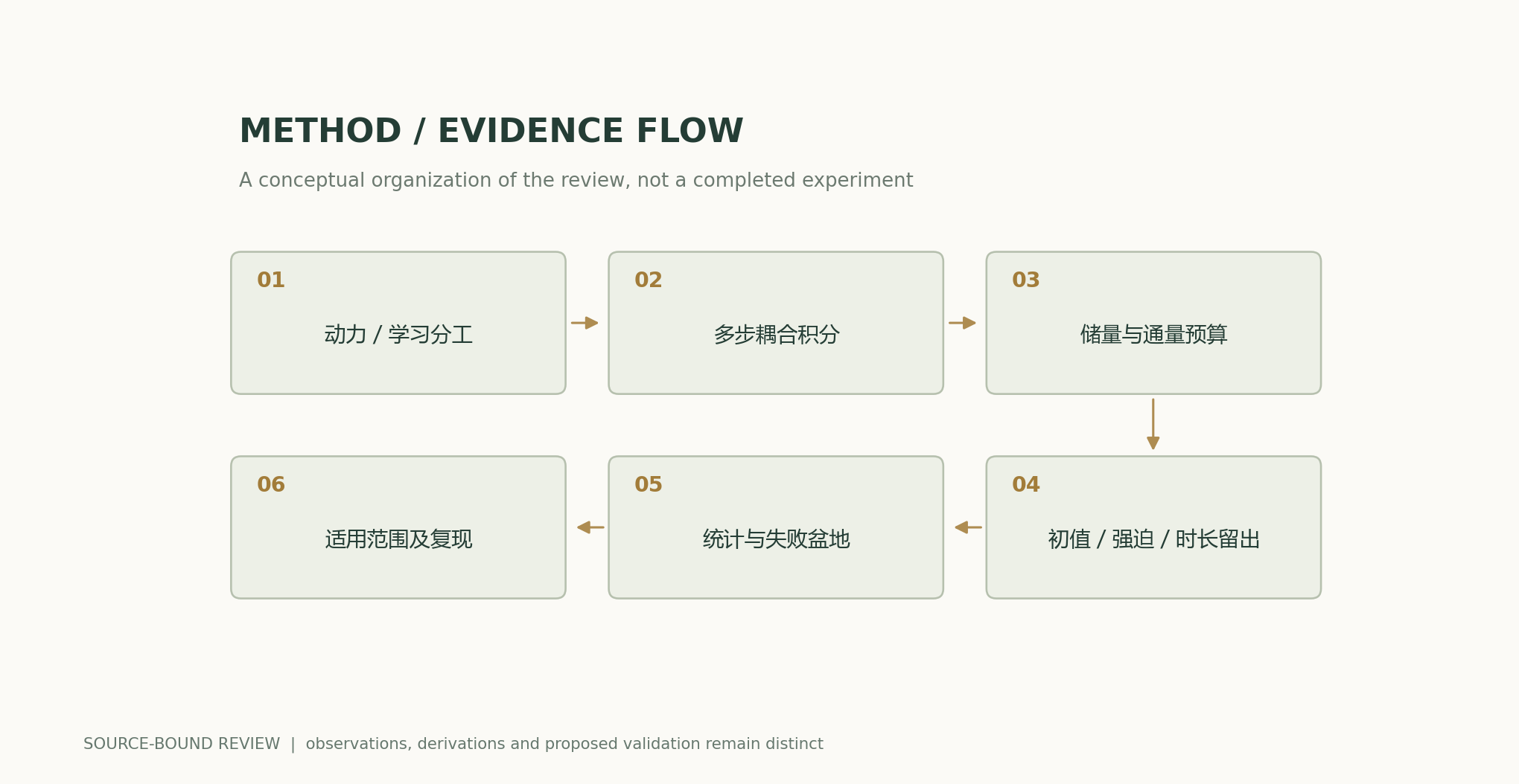
Analytical figures and numerical examples
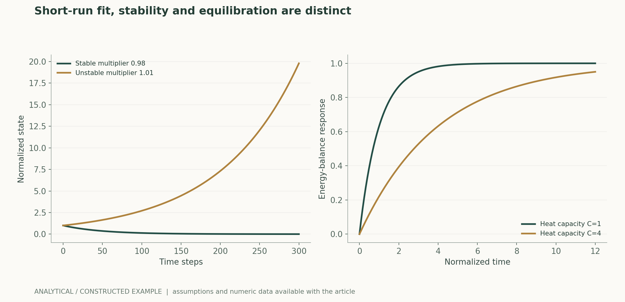
Recomputable worked example
From the same initial value, after 300 steps, 0.98^300≈0.002333, whereas 1.01^300≈19.7885. Both heat capacities lead to a long-term limit of 1, but their adjustment times differ; these parameters have no Earth-climate interpretation.
Method comparison
| Test axis | Explicit endpoint | Cannot establish |
|---|---|---|
| Short-term initial-value prediction | Lead-time error against a fixed analysis | Long-term stability |
| Multiyear statistics | Mean, variance, and seasonal cycle | Correct response to unknown forcing |
| Numerical stability | Completion rate across the full set of initial conditions | Valid conservation budgets |
| Energy and water budgets | Storage, fluxes, and residuals | Correct representation of all local phenomena |
| Prescribed sea-surface conditions | Atmospheric response with known boundaries | Fully coupled ocean–atmosphere prediction |
| Extrapolation to new forcing | Response magnitude and adjustment time | Reliability under any future scenario |
Verification and experimental plan
- Freeze the dynamical core, learned tendencies, grid, integrator, and forcing sources.
- Prespecify weather skill, long-term statistics, and forcing response as independent endpoints.
- Record energy, water, and mass budgets at every step, rather than saving only final fields.
- Use separate holdouts along the three axes of initial conditions, forcing, and duration.
- Fix the complete set of initial conditions and seeds, and include failed runs in the completion-rate denominator.
- Compare primary metrics on a common grid, and separately test local and extreme-event capabilities on native grids.
- Report training, tuning, and inference costs and actual product latency separately.
- Publish budgets and failed trajectories; do not register analytical energy-balance figures as actual climate projections.
Scope and limitations
- The scalar recurrence and energy-balance parameters in this article are all constructed examples.
- Neither NeuralGCM nor any real climate scenario was run.
- The linear-stability counterexample cannot quantify nonlinear atmospheric error.
- Prescribed-boundary simulations cannot replace fully coupled validation.
- Performance within the historical distribution is insufficient to guarantee reliability under substantially different future forcing.
Evidence from the original research and its scope
| Original research findings | Scope | Source and location |
|---|---|---|
| Combines a differentiable dynamical core with learned parameterizations and investigates weather and climate tasks. | Long-term settings include prescribed sea-surface conditions; the original paper limits extrapolation to substantially different future climates. | Neural general circulation models for weather and climateAbstract; Climate simulations; Methods |
| Compares multiple weather endpoints within a common evaluation framework. | Weather skill does not automatically validate climate feedback. | WeatherBench 2: A benchmark for the next generation of data-driven global weather modelsEvaluation design |
Research questions worth testing
- Which low-frequency modes are most sensitive to tiny biases in learned tendencies?
- Can explicit budget constraints improve stability under new forcing?
- Can models with equal weather skill produce substantially different long-term feedbacks?
Primary sources and corresponding claims
- Neural general circulation models for weather and climateKochkov et al. · 2024-07-22Differentiable hybrid atmospheric model; prescribed sea-surface temperatures; future-climate extrapolation limitation.
- WeatherBench 2: A benchmark for the next generation of data-driven global weather modelsRasp et al. · 2023-08-29Primary benchmark specification: initialization, regridding, reference analyses and multiple diagnostic metrics.
- Probabilistic weather forecasting with machine learningPrice et al. · 2024-12-04Abstract; 2019 test period, 50-member comparison, CRPS scorecard and dependent verification targets.
Citation and article export
BibTeXRISCSL JSONTXTArticle JSON
Author, version, and sources
A sourced research review and original analysis written by Codex (AI). Experiments in the original paper belong to the original research team; calculations in this article test only the listed equations and explicitly stated assumptions. This site does not yet have an independent peer review of this article or records of original model, clinical, or physical experiments for it.
First published: in-depth feature on AI and scientific discovery; preserves section-by-section sources and the distinction between original research evidence and the author’s analysis.
The conceptual cover was generated by ImageGen. Scientific figures were produced using the accompanying code and numerical files; captions specify assumptions and measurement definitions item by item.
Sources of the cover and scientific figures · Data, sources, and assumptions · Python · Code for recomputation · Publication and version history
Source revision: b7b48f7205d705b2a3d3e8de0be5e1b458e4869c