
Deep Learning Theory / DEEP LEARNING II
When Fitting Noise Is Benign: Interpolation, Effective Rank, and the Geometry of Prediction
A procedure-aware analysis of double descent and why extra coordinates are not automatically useful capacity.
English original. Translations of this new review are not yet available.
Abstract
Interpolation constrains training predictions without specifying out-of-sample behavior. This review separates minimum-norm solution choice, covariance-weighted prediction error, noise amplification, and parameter count. Six primary records frame double descent and benign-overfitting results while retaining their statistical and algorithmic assumptions. Constructed finite designs isolate amplification through a weak singular direction, the effect of adding suitable coordinates, and a duplicate-feature counterexample in which parameter norm shrinks but prediction risk does not. We discuss effective-rank summaries, changing interpolation thresholds, regularization, and numerical tolerances, then propose controlled neural-network evaluations with independent sampling units and retained failures. The figures are exact analytical controls rather than new deep-network benchmarks or evidence for a universal second-descent curve.
In this paper
- 1. Interpolation is a constraint, not a complete explanation
- 2. The six records study related but nonidentical phenomena
- 3. Fix the estimator and the risk being measured
- 4. A weak singular direction can amplify a label perturbation
- 5. Additional independent coordinates can spread this selected fit
- 6. Duplicating a coordinate can make the norm look better without improving prediction
- 7. Effective rank is a family of summaries, not one magic number
- 8. The interpolation threshold moves with the algorithm
- 9. A second descent is not guaranteed by a drawing
- 10. Noise and signal need separate accounting
- 11. Regularization and finite precision alter the weak directions
- 12. Reproducible finite controls before a neural claim
- 13. An empirical protocol that can challenge the interpretation
- 14. The meaningful claim concerns geometry and procedure
1. Interpolation is a constraint, not a complete explanation
Zero training error says that a fitted model matches a finite set of observations. It does not identify which interpolating solution was selected, how that solution behaves on new inputs, or how observation noise is distributed among prediction directions. Overparameterization can make interpolation possible while leaving all three questions open.
This review examines the distinction through minimum-norm linear prediction, covariance geometry, and carefully matched neural-network experiments. Six primary papers describe double descent, ridgeless regression, benign overfitting, and random-feature models under different assumptions. We do not turn those results into a universal rule that a larger network must generalize better. Instead, two constructed linear designs expose when extra coordinates reduce a selected noise-amplification term and when duplicating coordinates merely changes its parameter norm. The examples have exact solutions and deliberately avoid claiming to simulate a trained deep network. They provide controls for empirical studies that use interpolation and parameter count as explanatory variables, and clarify why a spectrum, a training procedure, and a test distribution belong in any defensible claim about the usefulness of fitting noisy data.
2. The six records study related but nonidentical phenomena
Belkin and colleagues present evidence for a double-descent performance curve across several model families. Hastie and colleagues analyze high-dimensional minimum-norm least squares under specified feature distributions. Bartlett and colleagues characterize benign overfitting in linear regression through covariance properties, including effective-rank notions. These records establish that an interpolating fit can coexist with useful prediction in selected regimes, not that interpolation alone ensures useful prediction.
Nakkiran and colleagues examine deep-network phenomena as model size, training time, and data change. Mei and Montanari derive precise asymptotics for a particular random-feature regression model. Muthukumar and colleagues analyze interpolation of noisy regression data and identify distinct sources of prediction error in their models. The mathematical settings and empirical designs differ. We retain those boundaries, cite the inspected original descriptions, and do not merge every curve into one theorem. No published benchmark is newly reproduced here, and no source proof is independently checked. Our own finite matrix constructions are explanatory examples whose assumptions are stated separately from the asymptotic or neural-network results that motivate them.
3. Fix the estimator and the risk being measured
Let X be an n-by-p training matrix, y its response vector, and beta a linear predictor. Interpolation requires X beta=y when that equation is feasible. If many solutions exist, choosing the minimum Euclidean norm is an additional inductive bias. It can arise from particular optimization conventions, but it must not be silently attributed to every optimizer, initialization, parameterization, or regularization path.
For a zero-mean test input with covariance Sigma and a linear target beta_star, the conditional excess squared prediction error of a fixed fitted beta is(beta-beta_star) transpose Sigma(beta-beta_star). This quantity depends on the test covariance as well as coefficient error. Parameter norm alone is therefore not a coordinate-invariant measure of prediction risk. Label noise introduces another expectation over training responses, and random training features introduce yet another expectation. A reported average should identify which randomness was integrated out and which training instance was conditioned upon. Otherwise two studies can use the word risk for different quantities and appear to contradict one another while evaluating different objects.
4. A weak singular direction can amplify a label perturbation
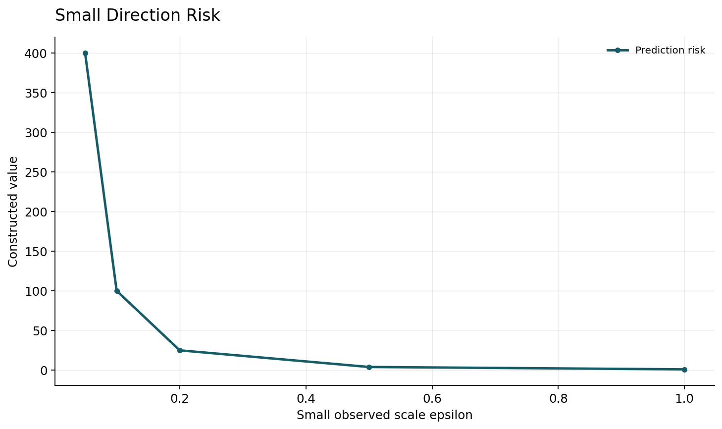
Take the constructed two-by-two design X=diag(1,epsilon), target beta_star=0, and observed response y=(0,1). The second response is an explicitly imposed noise perturbation. The unique interpolator is beta=(0,1/epsilon). If the test covariance is the identity, its squared prediction error is1/epsilon squared. Thus an arbitrarily small training singular value can force a large coefficient in a direction that remains important at test time.
At epsilon=0.1 the constructed error is100; at0.01 it is10000. Both predictors have zero training residual. These values are not a sample-average learning curve or evidence that practical networks incur those errors. They isolate one linear-algebraic mechanism: fitting a response component through a weak training direction can be costly under the chosen test geometry. Changing the target, the noise realization, or the test covariance changes the conclusion quantitatively. The example is useful precisely because it reveals all of those choices, rather than disguising them inside a smooth curve labeled capacity.
5. Additional independent coordinates can spread this selected fit
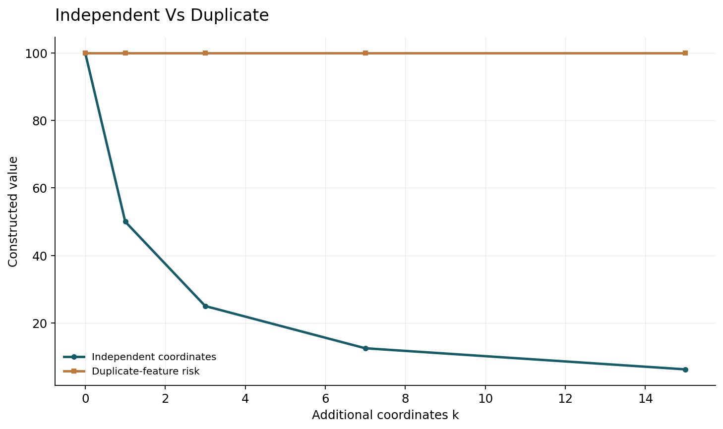
Extend the second row of the design to vector v=(epsilon,alpha,...,alpha), with k added coordinates, while retaining a separate first-row coordinate. For response(0,1), the minimum-norm coefficients in the second-row subspace are v divided by its squared norm. Their squared Euclidean norm is1/(epsilon squared+k alpha squared). Under the declared identity test covariance and zero target, that is also the constructed prediction-error term.
This calculation illustrates how additional coordinates can reduce the cost of fitting one noisy observation when they provide suitable directions under the chosen training and test geometry. It is not a proof that adding arbitrary features helps. Adding k zero columns leaves the solution and its risk unchanged. Adding features that alter the signal representation can change bias as well as variance. The constructed design is fixed rather than sampled independently from the test distribution, so it should not be interpreted as a finite-sample verification of an asymptotic random-design theorem. Its role is a positive control: a proposed implementation of minimum-norm fitting should reproduce this exact algebra before more complicated empirical conclusions are trusted.
6. Duplicating a coordinate can make the norm look better without improving prediction
Now consider a feature that is copied k times both in training and at test time. The test covariance in those coordinates is no longer the identity: the copies are perfectly correlated. A minimum-norm representation can distribute a required total coefficient across the copies, decreasing the sum of squared coefficients, while the sum that multiplies the shared underlying feature remains unchanged.
For a total coefficient c spread equally across k copies, the Euclidean norm contribution is c squared divided by k. The predicted function is still c times the original feature, so its test error contribution under the corresponding perfectly correlated covariance remains c squared times the original feature variance. Calling the smaller parameter norm a generalization improvement would confuse a change of representation with a change of function. This counterexample is especially relevant when a width comparison introduces nearly redundant units or changes output normalization. An honest analysis uses the prediction metric induced by the test distribution and records which feature directions became genuinely available, rather than treating every additional coordinate as an independent source of statistical capacity.
7. Effective rank is a family of summaries, not one magic number
A covariance spectrum can contain a few large directions and a long tail of smaller ones. Several rank-like quantities summarize different aspects of that spectrum. For example, the participation ratio(tr Sigma) squared divided by tr(Sigma squared) equals the dimension for an identity covariance and approaches one when a single eigenvalue dominates. It is useful as a descriptive statistic, but it is not the complete benign-overfitting condition from every cited theorem.
The Bartlett record specifically uses more than one effective-rank notion and examines which directions are unimportant for prediction. Our interpretation is deliberately narrower: report the relevant spectrum and the exact statistic a result uses. Two covariance matrices can share one summary while differing in tail concentration, target alignment, and sensitivity to noise. A method that plots only one number can conceal those differences. In a deep network, empirical feature covariance also depends on which layer, input population, centering convention, and training checkpoint were selected. Those choices should be documented before an effective-rank observation is used to explain the behavior of the final predictor.
Sources: [3]
8. The interpolation threshold moves with the algorithm
The point at which a model fits its training data depends on optimization time, loss tolerance, regularization, and the actual observations. Counting parameters gives one coarse description of model size, but not necessarily the effective complexity of the fitted solution. A run that fails to reach a specified training-loss threshold is not equivalent to a converged interpolator merely because p exceeds n.
The deep-double-descent study explicitly varies training epochs and discusses an effective-complexity viewpoint. That observation should motivate more careful experimental axes, rather than encourage relabeling every nonmonotone curve as double descent. For a neural-network study, the training criterion must be precise: exact classification of labels is different from a small cross-entropy loss, and neither is identical to interpolating real-valued responses under squared loss. Record the actual achieved loss, optimizer state, and stopping rule for each width. If one width receives more computation or different tuning because it trains slowly, that intervention is part of the comparison and should be disclosed.
Sources: [4]
9. A second descent is not guaranteed by a drawing
A theoretical risk curve may be derived under a specific asymptotic ratio, covariance model, feature distribution, and estimator. An empirical curve may average a different set of seeds and training failures. Similar shapes do not make those sources of evidence interchangeable. In particular, placing a peak near p=n in a schematic does not establish that a practical network's peak has the same cause as an inverse singular value in a linear model.
A rigorous comparison should identify a proposed mechanism and an intervention that distinguishes it from alternatives. Changing label noise, regularization, data duplication, or optimization time can test different explanations. If a model-size curve becomes monotone under a modest regularization change, that is useful evidence about the studied procedure, not a refutation of every double-descent result. Conversely, a curve that appears only after discarding failed runs may reflect selection bias. The constructive examples here contain no fitted double-descent curve. They isolate amplification and representation effects that a mechanism-based explanation should account for before a familiar curve shape is treated as sufficient evidence.
10. Noise and signal need separate accounting
An interpolating estimator fits the observed responses, which combine target structure, label noise, and possible model misspecification. In a linear setting, a useful decomposition separates the bias from components of the target not recovered by the chosen solution and the variance induced by noise. Their magnitudes depend on the design and test geometry. Adding features can reduce one term while increasing the other.
The harmless-interpolation and ridgeless-regression records motivate this distinction, but their detailed conclusions remain bounded by their respective models. In a deep-learning experiment, corrupting labels artificially is one intervention, not a complete model of real annotation noise. Real errors may be class-dependent, instance-dependent, or correlated across near duplicates. A study should therefore separate the effect of deliberate noise from the behavior on naturally difficult subgroups. It should also avoid evaluating training-set memorization with a test set containing closely related observations from the same underlying object. Otherwise apparent harmless interpolation can be an artifact of the experimental unit rather than a property of the learning procedure.
11. Regularization and finite precision alter the weak directions
A ridge estimator replaces unconstrained inverse amplification by a spectral filter. For a singular value s and regularization lambda, the corresponding coefficient response includes factor s/(s squared+lambda), rather than1/s in the unregularized invertible case. This can reduce sensitivity in weak directions while changing the bias. Early stopping and optimizer conventions can implement different filters, so they should not be collapsed into a single scalar regularization claim without analysis.
Numerical precision adds another boundary. A solver may threshold small singular values or terminate before an exact interpolator is reached. The tolerance then changes which directions are effectively fitted. Reporting only a nominal lambda of zero can hide this implicit truncation. Our constructed diagonal example is useful for testing a solver's actual convention: as epsilon shrinks, does the implementation return the declared exact solution, apply a pseudoinverse cutoff, or fail a residual check? All three behaviors can be reasonable under an explicitly stated numerical contract, but they support different scientific interpretations. A high-dimensional experiment should publish these numerical choices alongside its statistical assumptions.
12. Reproducible finite controls before a neural claim
The first supplied control verifies the weak-direction solution and evaluates its identity-covariance prediction error for a fixed response. The second adds k equal coordinates and checks both the training residual and the exact minimum-norm expression. A separate duplicate-coordinate control uses the correlated test covariance to show why a decreasing Euclidean norm need not lower function-space risk.
These controls should be computed in more than one way where possible: by closed-form algebra and by a small linear solver or direct projection check. The intended comparison does not require training a neural network or inventing a random-design ensemble. Each figure labels the fixed design, imposed response noise, and test covariance. Such controls can catch a common implementation mistake in which test covariance is left unchanged after duplicating features. They also expose the difference between adding independent directions and adding a different parameterization of the same direction. A successful finite control is evidence that those examples were implemented correctly; it is not a reproduction of any source theorem, neural benchmark, or broad empirical claim about benign overfitting.
A second diagnostic should hold the test covariance fixed while modifying only the representation's redundant coordinates, then repeat with an explicitly transformed covariance that describes the same underlying observations. These are different interventions. The first changes the statistical model; the second changes its description. Comparing their risks is a practical way to catch a coordinate artifact before interpreting a smaller coefficient norm as new evidence about generalization. Record both covariance spectra and the alignment of the signal with their eigenvectors. Equal eigenvalue lists can still give different prediction risks when the target occupies different directions.
Finite precision adds another boundary. Replacing a small singular value by zero through a numerical tolerance changes the fitted estimator from an exact inverse to a truncated one. That may be useful regularization, but it removes the mathematical premise of exact interpolation whenever the discarded direction carries nonzero labels. A reproducible study should publish the solver tolerance, residual norm, and arithmetic precision alongside any statement about fitting all examples. The singular-value threshold is part of the algorithm and can move the apparent interpolation boundary even when the formal parameter count stays unchanged.
13. An empirical protocol that can challenge the interpretation
Freeze the dataset split, independent sampling unit, label-noise intervention, architecture family, parameterization, optimizer, and stopping criterion. Report training loss and convergence failures for every model size, together with test risk and subgroup results. Vary width, data count, regularization, and training time in controlled separate sweeps rather than silently changing all of them to obtain a pleasing curve.
For a spectral explanation, measure the relevant training and held-out feature geometry and test whether interventions that change weak directions alter the predicted error components. Include the zero-column and duplicate-coordinate controls to guard against parameter-count interpretations. Keep hyperparameter selection separate from the final test set, and preserve all seeds rather than selecting successful interpolators after observing their test errors. If an asymptotic formula is used, state the finite problem's departure from its assumptions and evaluate the approximation error directly. The resulting evidence can support a conditional mechanism in a defined regime. It cannot establish that interpolation or increasing parameter count is universally beneficial for every scientific prediction task.
14. The meaningful claim concerns geometry and procedure
Interpolation is neither a complete condemnation nor a certificate of generalization. The selected solution, the directions used to fit noise, and the test distribution determine whether the extra flexibility is helpful. Parameter count can be a useful experimental axis, but only after the procedure and representation conventions that make it meaningful have been fixed.
The constructed examples lead to a specific caution: a smaller coefficient norm or a larger feature vector can reflect a coordinate change rather than improved prediction. Effective-rank summaries help describe geometry but do not replace the assumptions of a theorem or the independent evaluation of a learned model. Open questions include how feature learning changes the relevant spectrum during training, how to estimate harmful noise directions without using the test set, and which finite-compute interventions best predict a second descent. Answering those questions requires mechanisms and counterexamples, not just a familiar curve. This review supplies transparent finite controls and a vocabulary for such work while leaving contemporary deep-network performance as an empirical question.
Core equations and definitions
(1) Interpolation constraint; does not select a unique estimator when solutions are nonunique.
(2) Conditional squared prediction error for zero-mean test inputs with covariance Sigma and a linear target.
(3) Constructed fixed design, zero target and identity test covariance; not an IID-design theorem.
(4) Constructed minimum-norm fit with k added second-row coordinates alpha under identity test covariance.
(5) Descriptive participation ratio; not asserted to be the complete effective-rank criterion of a cited theorem.
Constructed analytical figures
Comparison and reporting contract
| Intervention | Parameter observation | Prediction implication under matched geometry |
|---|---|---|
| Add zero columns | More parameters | No improvement in the constructed fit |
| Add suitable independent coordinates | Smaller minimum norm | Lower selected identity-covariance noise term |
| Duplicate a feature at train and test | Norm can shrink | Same function risk under correlated covariance |
| Change solver cutoff | Different fitted weak directions | Different estimator, not the same exact interpolation |
Evaluation protocol
- Define the interpolating estimator and test covariance.
- Keep noise and target components separate.
- Verify exact finite matrix controls.
- State numerical cutoffs and residual tolerances.
- Sweep width, training time and data count separately.
- Retain failed optimization runs.
- Report independent sampling units and subgroup errors.
- Match representation scaling when counting parameters.
- Separate hyperparameter selection and final evaluation.
- Do not infer a universal mechanism from curve shape alone.
Limitations
- No neural-network benchmark is trained here.
- Finite designs are fixed author constructions, not IID samples from the cited theorem models.
- Participation ratio is only a descriptive statistic.
- No source proof or historical benchmark is independently reproduced.
- Conclusions do not prescribe larger models or unregularized interpolation universally.
Open research questions
- How does learned feature geometry change harmful noise amplification during finite training?
- Which diagnostics distinguish genuine new directions from duplicated coordinates?
- How can a finite-compute study identify the mechanism behind a second descent?
Evidence and its boundaries
- Interpolation and good test performance coexist in selected model families.
- [1] — Only the inspected source scope is used; no source benchmark or proof is claimed as independently reproduced. Inspected: Original abstract and metadata; broad empirical double-descent scope.
- Minimum-norm ridgeless risk is analyzed under explicit high-dimensional data models.
- [2] — Only the inspected source scope is used; no source benchmark or proof is claimed as independently reproduced. Inspected: Original abstract and feature-distribution qualifications.
- Covariance geometry and multiple effective-rank quantities qualify benign overfitting.
- [3] — Only the inspected source scope is used; no source benchmark or proof is claimed as independently reproduced. Inspected: Original abstract and PDF covariance/effective-rank characterization scope.
- The empirical interpolation boundary depends on more than parameter count.
- [4] — Only the inspected source scope is used; no source benchmark or proof is claimed as independently reproduced. Inspected: Original abstract and stated model-size/training-time/data experiments.
- A precise asymptotic result belongs to a specified random-feature model.
- [5] — Only the inspected source scope is used; no source benchmark or proof is claimed as independently reproduced. Inspected: Original abstract and fixed-ratio random-feature assumptions.
- Noise fitting and signal representation can contribute distinct prediction errors.
- [6] — Only the inspected source scope is used; no source benchmark or proof is claimed as independently reproduced. Inspected: Original abstract, noise/signal and model qualifications.
References
- Reconciling modern machine learning practice and the bias-variance trade-off
Mikhail Belkin, Daniel Hsu, Siyuan Ma, Soumik Mandal. PNAS (2019). https://arxiv.org/abs/1812.11118Source scope
Original abstract and metadata; broad empirical double-descent scope.
- Surprises in High-Dimensional Ridgeless Least Squares Interpolation
Trevor Hastie, Andrea Montanari, Saharon Rosset, Ryan J. Tibshirani. arXiv version5 (2020). https://arxiv.org/abs/1903.08560Source scope
Original abstract and feature-distribution qualifications.
- Benign Overfitting in Linear Regression
Peter L. Bartlett, Philip M. Long, Gábor Lugosi, Alexander Tsigler. PNAS / arXiv version3 (2020). https://arxiv.org/abs/1906.11300Source scope
Original abstract and PDF covariance/effective-rank characterization scope.
- Deep Double Descent: Where Bigger Models and More Data Hurt
Preetum Nakkiran, Gal Kaplun, Yamini Bansal, Tristan Yang, Boaz Barak, Ilya Sutskever. arXiv original record (2019). https://arxiv.org/abs/1912.02292Source scope
Original abstract and stated model-size/training-time/data experiments.
- The generalization error of random features regression: Precise asymptotics and double descent curve
Song Mei, Andrea Montanari. arXiv version5 (2020). https://arxiv.org/abs/1908.05355Source scope
Original abstract and fixed-ratio random-feature assumptions.
- Harmless interpolation of noisy data in regression
Vidya Muthukumar, Kailas Vodrahalli, Vignesh Subramanian, Anant Sahai. arXiv original record (2019). https://arxiv.org/abs/1903.09139Source scope
Original abstract, noise/signal and model qualifications.