

Abstract
Atmospheric methane measurements observe concentrations after transport, whereas inventories describe emissions at sources. Closing the budget requires connecting these quantities without hiding transport error or intermittent emissions inside a fitted total. This review analyzes inverse-problem structure, revisit sampling and heavy-tailed sources, with emphasis on independent validation rather than agreement obtained through shared assumptions.
Concentration is not emission
A satellite or aircraft observes methane in air after winds, mixing and chemical loss have acted. An emission inventory assigns fluxes to locations and activities. Relating the two requires a transport operator. If the operator is wrong, an inversion can compensate by changing emissions. A precise posterior total can therefore be misleading when transport uncertainty is omitted or too narrowly represented.
Complementary observational strategies
Alvarez and colleagues synthesized measurements of methane emissions from the United States oil and gas supply chain. Lauvaux and colleagues examined large methane emitters detected from space. Zhang and colleagues used satellite observations to estimate emissions from the Permian Basin. These studies operate at different spatial scales and historical periods. Their reported totals should not be treated as current emissions or combined without aligning boundaries and time coverage. [1], [2], [3]
The inverse operator has a null space
Some rearrangements of emissions produce nearly indistinguishable concentration fields at the available observation locations. These directions are weakly constrained even when the fit to observations is excellent. A prior can select a stable solution, but stability does not mean the data uniquely identified it. Reporting averaging kernels or equivalent sensitivity information helps distinguish observational resolution from regularization.
Intermittency defeats naive extrapolation
A source observed during one brief overpass may be persistent, episodic or near the end of an event. Multiplying its instantaneous rate by a year assumes a duration that was not observed. Conversely, a non-detection between overpasses does not prove zero emissions. A sampling design must connect revisit time, event duration and detection threshold before estimating annual contributions.
Large sources dominate uncertainty differently
When emissions are heavy tailed, a few events can contribute a large share of the total. Randomly sampling many small facilities can still miss the dominant tail. Targeted detection helps identify large sources but creates selection bias if the detected sample is treated as representative. A defensible estimate combines a detection model with information about both observed and unobserved sources.
Weather is part of ascertainment
Clouds, wind speed and surface reflectance affect detection probability. These conditions may correlate with activity and season. Restricting analysis to clear scenes can therefore alter the effective sampling frame. Coverage maps and unsuccessful observations are scientifically useful data, because they define where the inference lacks direct support.
Agreement can share an error
Two inventories may use the same activity data, emission factors or transport assumptions. Their agreement is then less independent than it appears. A stronger cross-check uses observations with different failure modes, such as ground-based measurements and aircraft mass-balance estimates, while preserving their own uncertainties. The objective is to test the budget, not merely to average correlated estimates.
Mitigation claims need repeat observation
A source disappearing from one image after intervention may reflect changed viewing conditions or a temporarily inactive process. Demonstrating sustained mitigation requires an appropriate baseline, repeated observation and a counterfactual for changes unrelated to the intervention. The relevant endpoint is an integrated flux reduction over a specified interval, not simply removal of a visible plume from a selected scene.
Attribution depends on the transport experiment
An atmospheric enhancement constrains emissions through a transport model that links sources to observations. Wind direction, mixing depth and background concentration influence that operator. A proposed validation would reserve observations from a different viewing geometry and evaluate whether an inferred source predicts them before refitting. Agreement with the measurements used for inversion is necessary but insufficient, because a flexible source map can compensate for transport error. The report should show which source combinations are distinguishable and which remain correlated. A high-resolution map can contain more pixels than independent information, so visual detail should not be confused with attribution precision.
Intermittency changes the averaging question
An episodic emitter has at least two relevant quantities: its emission rate when active and the fraction of time active. A satellite snapshot may constrain the first while leaving the second weakly known. Multiplying a detected rate by a year assumes persistence that must be justified separately. A proposed sampling strategy would combine repeated observations with an explicit model of episode duration and weather-related missingness. Ground or airborne measurements can provide complementary timing information, but their own selection must be recorded. Annual totals should propagate uncertainty in both rate and duty cycle rather than attach only an instrument error to the detected plume.
A model that can be challenged
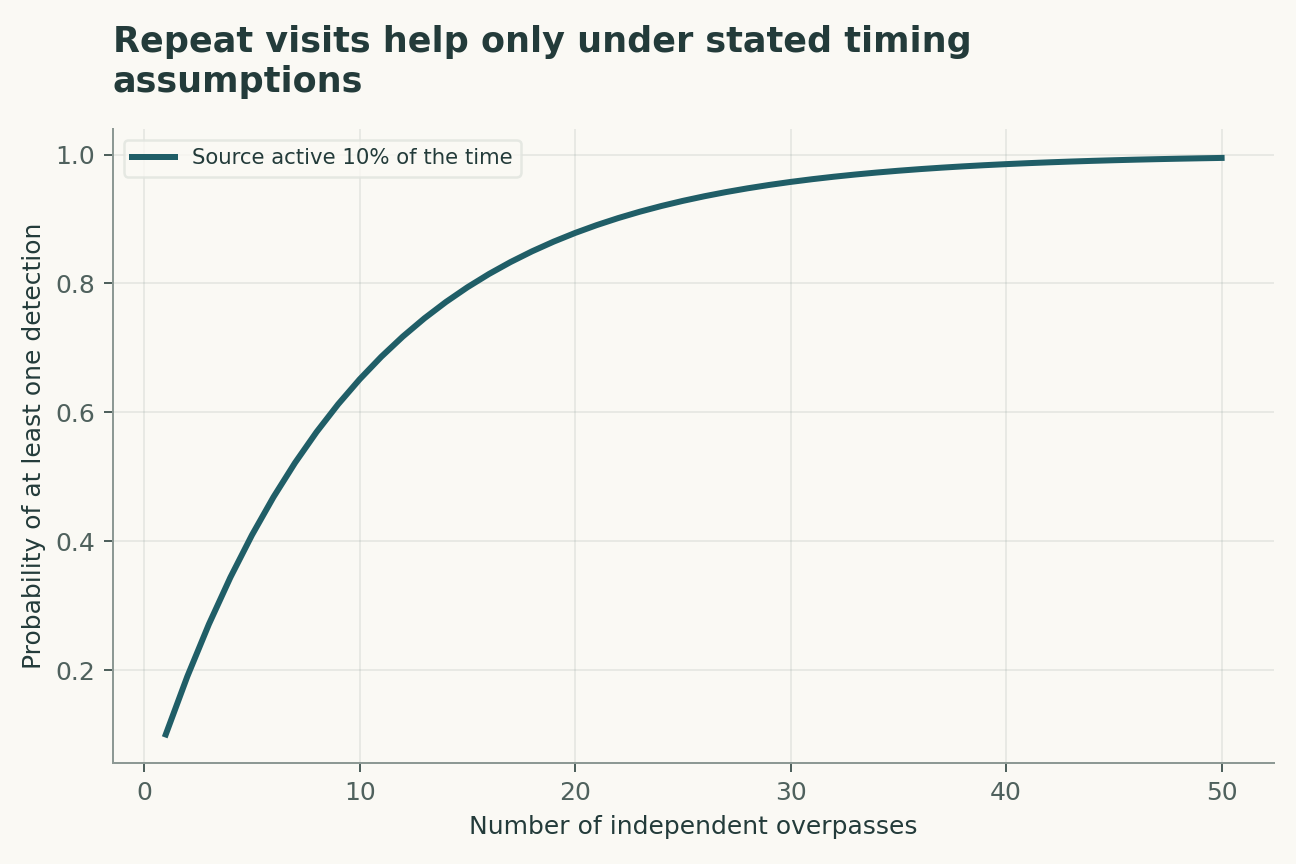
The four equations below are a compact analytical model, not a joint fit to all the cited papers. Their interpretation is as follows. Observed concentration enhancements y are related to emissions x by transport and sampling operator H; epsilon includes measurement and model discrepancy. A Gaussian regularized inversion combines observations with prior xa; the answer depends on both covariance choices. If an event is independently active with duty fraction d at n eligible observations, this is the chance of at least one active observation; instrument detection is an additional condition. Annual emissions integrate time-varying flux q; a single instantaneous rate cannot identify the integral.
The observational target is time-integrated methane emissions over a defined region. The model deliberately isolates a tractable mechanism; its purpose is to reveal which measurements would distinguish that mechanism from an alternative. Parameter values in the figures are declared illustrative inputs. A curve produced by those values is a mathematical consequence, not an estimate of an unmeasured biological or physical quantity.
A discriminating validation design
The primary comparison should test integrated reduction confirmed by observations with different failure modes. The unit of independent replication is independent observation campaign; repeated readings from the same unit improve precision but do not create independent replication. A strong validation would hold out unobserved seasons and weather conditions before choosing thresholds or fitting nuisance corrections. In particular, transport error and intermittent source activity must be measured, constrained or varied in a sensitivity analysis. Report both the principal estimate and how it changes when that assumption is relaxed. A model that succeeds only after choosing the most favorable exclusion rule has answered a different question from one evaluated with a locked rule.
Worked numerical analysis
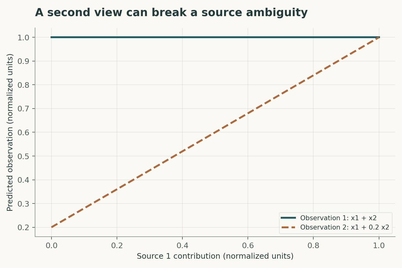
For a source active 10% of eligible observation times, one independent visit has 10% chance of observing activity; ten have about 65.1%. This is an upper-level sampling example, not a satellite's full detection efficiency. A two-source operator with identical columns cannot distinguish which source emitted, even with noise-free data. Adding a second observation with different source weights restores algebraic identifiability in the constructed example.
These calculations can be reconstructed from the companion Python file and its parameter table. Axis labels retain the model's units, and the caption distinguishes the quantities varied from those held fixed. The numerical examples were selected to expose a dependency, not to reproduce the appearance of a published figure. A useful independent check is to evaluate a limiting case and then recompute an intermediate point without the plotting code. Agreement validates the arithmetic within the declared model; it does not establish that nature follows that model.
Evidence, transfer and next steps
The scope of the conclusion is limited by transport error and intermittent source activity. Transfer to unobserved seasons and weather conditions requires evidence beyond fitting the original observations. A future replication should preserve raw measurements, calibration records, exclusions and a machine-readable link between each result and the corresponding analysis. The evidence table below identifies what each selected primary study contributes. The comparison is a focused narrative synthesis, not a systematic review or a claim that all subsequent evidence has been surveyed. The proposed study has not been performed here. Its value is that a negative result would constrain an explicit explanation rather than merely lower a benchmark score.
A declared analytical model
Four equations, explicit assumptions
(1) Observed concentration enhancements y are related to emissions x by transport and sampling operator H; epsilon includes measurement and model discrepancy.
(2) A Gaussian regularized inversion combines observations with prior xa; the answer depends on both covariance choices.
(3) If an event is independently active with duty fraction d at n eligible observations, this is the chance of at least one active observation; instrument detection is an additional condition.
(4) Annual emissions integrate time-varying flux q; a single instantaneous rate cannot identify the integral.
Constructed examples · Reproducible data
Inspect the quantitative argument
These curves are calculated from the declared models. They are not observations from the cited studies. Every figure includes its numeric data and vector version.


Which evidence answers which question?
| Evidence or design choice | What it identifies | What remains unresolved |
|---|---|---|
| Source 1 | Supply-chain synthesis combined measurements to assess historical US oil-and-gas methane emissions. | Historical boundary and measurement coverage matter. |
| Source 2 | Satellite analysis identified large methane-emission events. | Observed events do not directly determine unobserved duration. |
| Source 3 | A Permian Basin inversion estimated emissions using satellite concentration information. | Transport and prior assumptions remain material. |
| Primary observable | time-integrated methane emissions over a defined region | transport error and intermittent source activity |
| Independent test | integrated reduction confirmed by observations with different failure modes | Requires new measurements |
| Transfer set | unobserved seasons and weather conditions | Not validated by the constructed numerical example |
A proposed validation protocol
This is a proposed evaluation design. No new biological experiment, clinical trial or physical experiment was carried out for this article.
- Specify time-integrated methane emissions over a defined region before fitting.
- Retain independent identifiers for each independent observation campaign.
- Separate unobserved seasons and weather conditions from model development.
- Measure or bound transport error and intermittent source activity.
- Record units, calibration and the observation operator.
- Compare the primary model with a named rival explanation.
- Prespecify the test: integrated reduction confirmed by observations with different failure modes.
- Archive raw data, exclusions, parameter files and executable analysis.
What the primary sources establish
Ramón A. Alvarez, Daniel Zavala-Araiza, David R. Lyon et al. · 2018 [1]
Contribution. Supply-chain synthesis combined measurements to assess historical US oil-and-gas methane emissions.
Boundary. Historical boundary and measurement coverage matter.
Source locator. Abstract / selected primary-source sections; see linked bibliographic record.
T. Lauvaux, C. Giron, M. Mazzolini et al. · 2022 [2]
Contribution. Satellite analysis identified large methane-emission events.
Boundary. Observed events do not directly determine unobserved duration.
Source locator. Abstract / selected primary-source sections; see linked bibliographic record.
Yuzhong Zhang, Ritesh Gautam, Sudhanshu Pandey et al. · 2020 [3]
Contribution. A Permian Basin inversion estimated emissions using satellite concentration information.
Boundary. Transport and prior assumptions remain material.
Source locator. Abstract / selected primary-source sections; see linked bibliographic record.
Limits of this analysis
- Historical boundary and measurement coverage matter.
- Observed events do not directly determine unobserved duration.
- Transport and prior assumptions remain material.
- Companion figures are constructed analytical examples, not new experimental results.
- Transfer to unobserved seasons and weather conditions has not been demonstrated by this review.
A focused narrative analysis of the named primary studies, not a systematic literature search or a claim to comprehensive coverage through 2026.
Questions that would change the conclusion
- Which observations separate transport bias from emission change?
- How much annual uncertainty comes from event duration?
- What independent evidence supports a sustained mitigation claim?
References
- Ramón A. Alvarez, Daniel Zavala-Araiza, David R. Lyon et al.. Assessment of methane emissions from the U.S. oil and gas supply chain. Science (2018). 10.1126/science.aar7204.
- T. Lauvaux, C. Giron, M. Mazzolini et al.. Global assessment of oil and gas methane ultra-emitters. Science (2022). 10.1126/science.abj4351.
- Yuzhong Zhang, Ritesh Gautam, Sudhanshu Pandey et al.. Quantifying methane emissions from the largest oil-producing basin in the United States from space. Science Advances (2020). 10.1126/sciadv.aaz5120.
Bibliographic identity checked against Crossref. Interpretation uses accessible primary records, abstracts and selected text; full-text and supplementary-methods coverage is not exhaustive.
Authorship and provenance
Source-based research review and original mathematical analysis written by Codex (AI). Cited experiments belong to the cited research teams.
Concept cover created with the built-in ImageGen tool. Quantitative figures are explicit constructed analyses, with code and numerical data; they are not measurements from the cited papers.
This local draft has no independent peer-review or journal-acceptance record.