
Architectures & Continuous Models / DEEP LEARNING II
The Solver Is Part of the Network: Neural ODEs, Discrete Gradients, and Numerical Fidelity
A continuous-time model becomes an executable predictor only after a solver, tolerances, interpolation and gradient strategy have been specified.
English original. Translations of this new review are not yet available.
Abstract
Neural ordinary differential equations parameterize a hidden-state derivative rather than a fixed sequence of layers. Their executable behavior nevertheless depends on a numerical method, stopping rules and differentiation choices. This review connects six primary sources on neural ODEs, discrete-gradient accuracy, state augmentation, regularization, adjoint error control and controlled differential equations. An analytically solvable scalar system separates the exact flow from explicit Euler implementations: at a damping coefficient of minus two, one step reverses the state's sign, two steps collapse it to zero, and finer grids approach the positive exact solution. The exact derivative and the derivative of each discrete solver are computed separately. A second construction shows that stable forward contraction can amplify endpoint perturbations during backward reconstruction. These calculations are not benchmarks of any cited model. They expose why continuous-time expressiveness, numerical accuracy, training gradients and observed computation cost are separate claims. We propose evaluation across solver settings, state and gradient checks, observation interpolation and explicit failure budgets, with all quality comparisons tied to a frozen executable configuration.
In this paper
- 1. A differential equation is not yet a deployed predictor
- 2. What the original architecture changes
- 3. A scalar model separates exact and discrete behavior
- 4. The derivative of a solver is its own object
- 5. Reverse reconstruction can amplify small errors
- 6. Discretization-aware gradients clarify the target
- 7. Local error control is not a universal output guarantee
- 8. Adjoint error norms affect work allocation
- 9. State augmentation changes representational constraints
- 10. Regularization can alter the cost of solving
- 11. Observations require an input pathway
- 12. Function evaluations are a partial compute measure
- 13. A tolerance sweep is an intervention on the predictor
- 14. Reproducibility includes numerical configuration
- 15. What the constructed checks establish
- 16. Numerical fidelity is part of model identity
1. A differential equation is not yet a deployed predictor
A neural ODE describes how a hidden state changes with a continuous coordinate. A deployed program must still decide how to approximate that change, when to stop and how to handle a failed solve. The resulting predictor is therefore determined by parameters and an execution configuration together. Replacing a solver or tolerance can change outputs without changing a single learned weight.
This article examines that executable contract rather than treating numerical integration as an invisible implementation detail. The contract includes the initial-state map, derivative network, integration interval, arithmetic precision, solver, error-control rule and output map. Training adds another choice: which computational object is differentiated. A derivative of the exact flow, a derivative of a fixed numerical discretization and an approximation produced by a separate backward solve need not agree at a finite budget. These distinctions matter when comparing architectures or claiming efficiency. We use small solvable systems to isolate them without pretending that scalar calculations reproduce a high-dimensional learned model.
2. What the original architecture changes
Chen and colleagues parameterize the hidden-state derivative with a neural network and compute an output using an ODE solver. This replaces an explicitly listed layer sequence with a continuous-time description. The primary record inspected here includes a later correction note, so we identify the version and avoid reusing function-evaluation counts from an unspecified edition. The architectural idea does not require us to assume that every numerical approximation has the properties of the ideal flow.
The continuous description can make parameters reusable across integration settings, but an executable comparison must report the settings actually used. A coarse solve may resemble a shallow discrete network while a tighter solve can invoke the derivative many more times. The number of evaluations can vary with the input, learned dynamics and error-control policy. Consequently, parameter count alone does not determine inference cost. A fair baseline should compare quality under matched resource constraints and should state whether a solver change is considered a permissible deployment adjustment or a change to the predictor being evaluated.
Sources: [1]
3. A scalar model separates exact and discrete behavior
Consider the scalar differential equation dz/dt=theta times z, with z at time zero equal to one and the endpoint at time one. Its exact solution is the exponential of theta. Explicit Euler with N equal steps instead gives the product of N factors, each equal to one plus theta divided by N. Both formulas are elementary enough to evaluate and differentiate independently.
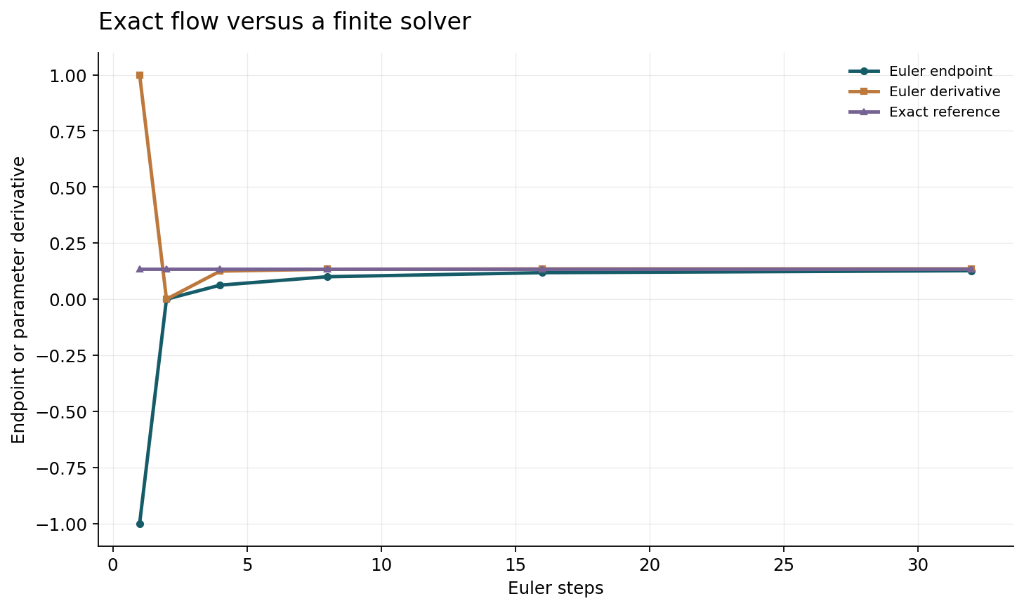
At theta equal to minus two, the exact endpoint is positive and approximately 0.135335. One Euler step gives minus one, reversing the sign. Two steps give zero. Four steps give 0.0625, eight give approximately 0.100113, and thirty-two give approximately 0.126789. These are not measured neural-network accuracies. They show that a finite discretization can produce qualitatively different behavior from a stable continuous system. Labeling every row as the same continuous-depth model would conceal the implementation choice that produced the difference. The example also supplies a regression case for solver wrappers: endpoint values, failures and settings can be checked against an analytic reference.
4. The derivative of a solver is its own object
For the scalar system, the exact derivative of the endpoint with respect to theta is again the exponential of theta. The derivative of the N-step Euler endpoint is the factor one plus theta divided by N raised to the power N minus one. At theta equal to minus two, the one-step derivative is one, the two-step derivative is zero and the four-step derivative is 0.125. These differ from the exact derivative even though they are correct derivatives of their respective discrete formulas.
This is the central distinction between differentiating a continuous mathematical model and differentiating the program used to approximate it. A training implementation should state which objective its gradient approximates. A gradient check using finite differences of the numerical program can validate consistency with that program, while comparison with an analytic flow derivative tests a different approximation. Both checks are useful. Passing one should not be described as passing the other. Adaptive step selection adds further implementation choices about how branch decisions in the solver are treated during differentiation.
5. Reverse reconstruction can amplify small errors
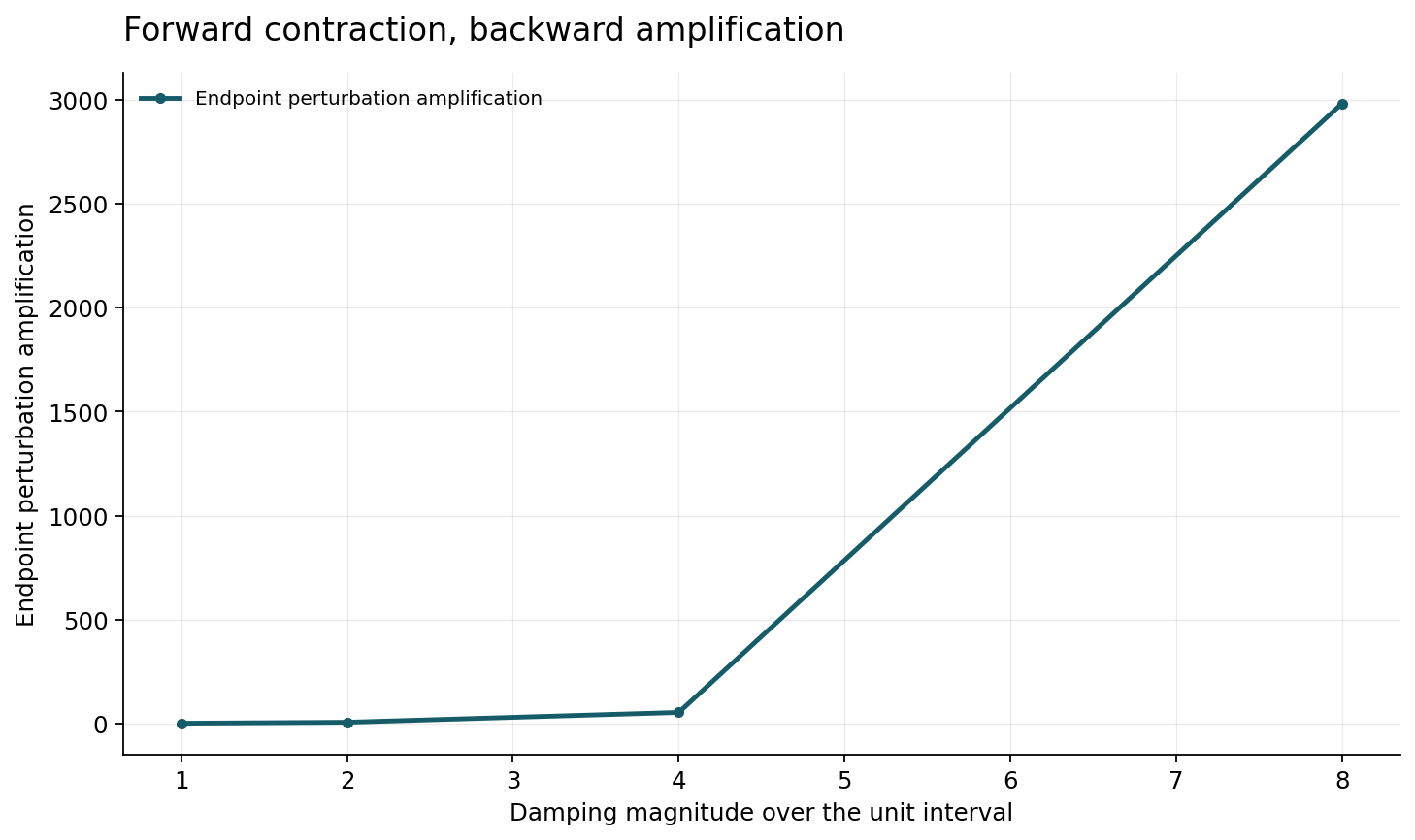
The exact scalar flow with theta negative contracts differences during forward integration. Reconstructing an initial state from the endpoint applies the inverse factor and amplifies endpoint perturbations. For damping magnitudes one, two, four and eight over a unit interval, the amplification factors are approximately 2.72, 7.39, 54.60 and 2980.96. Exact reversibility and numerical conditioning are therefore different properties.
A small endpoint error can become substantial during backward reconstruction even when the forward trajectory appeared well behaved. This does not prove that every adjoint calculation is unstable, nor does it invalidate continuous adjoint theory. It identifies a condition that an implementation must manage. Checkpointing can preserve intermediate forward states, while recomputation and tighter tolerances trade memory for additional work. The relevant experiment reports reconstruction error, gradient discrepancy and memory cost together. A claim of low memory usage should also define whether stored observations, solver workspaces, parameters and checkpoints are included, rather than counting only the hidden state.
6. Discretization-aware gradients clarify the target
ANODE discusses numerical problems associated with reverse reconstruction and inconsistency between optimization and discretization. Its methodological relevance is to make the gradient target explicit and to use stored or recomputed information in a controlled way. We do not interpret its title as a guarantee that every solver or arithmetic format returns a mathematically exact gradient.
The scalar example gives a simple diagnostic for this distinction. A method claiming to differentiate the chosen Euler implementation should match the closed-form discrete derivative and finite differences of the same implementation within a stated numerical tolerance. A method claiming to approximate the exact flow derivative should instead be compared with the exponential reference as the integration budget changes. If these tests use different endpoint programs, a mismatch cannot be interpreted cleanly. For real networks, exact references may be unavailable, but small analytically solvable subsystems and carefully tightened reference solves can still reveal whether an error originates in forward integration, reconstruction, automatic differentiation or the chosen continuous formulation.
Sources: [2]
7. Local error control is not a universal output guarantee
An adaptive solver typically compares an estimated local error with a scale determined by absolute and relative tolerances. The acceptance decision depends on the selected norm and on the components included in that norm. This is a numerical control mechanism, not a direct certificate that a downstream classification probability or generated sample is within the same tolerance of an ideal model.
The connection from state error to output error depends on the output map and the dynamics. A small state perturbation can be magnified by a sensitive readout. A seemingly generous relative tolerance can behave differently near zero, where an absolute component matters. A report should therefore identify both numerical tolerances and task-level deviations observed when those tolerances are changed. It should include unsuccessful solves and maximum-step events rather than dropping difficult inputs. For a fixed deployed configuration, those events are part of the predictor's service behavior. Calling them implementation noise hides exactly the cases in which numerical assumptions deserve the most attention.
8. Adjoint error norms affect work allocation
Kidger, Chen and Lyons show that the structure of adjoint equations can make a standard error-control norm unnecessarily restrictive for some components, motivating a seminorm. The inspected primary source supports the importance of the acceptance criterion. Its reported evaluation savings do not establish a universal reduction in latency, energy or gradient error for every application.
The broader lesson is that computation is allocated according to a numerical objective chosen by the implementation. If a component contributes to an error norm but is not needed to control a particular integration accuracy target in the same way, the solver may reject useful steps unnecessarily. Conversely, removing components without a justified analysis can under-control an error that matters. Evaluation should compare both the number and type of derivative evaluations, the resulting gradients and end-task outcomes. A derivative network can have different costs for different shapes or hardware kernels, so equal evaluation counts do not automatically imply equal wall-clock time. Warmup, batching and memory traffic remain separate empirical measurements.
Sources: [5]
9. State augmentation changes representational constraints
Dupont and colleagues analyze limitations of ordinary neural ODE representations and introduce augmented hidden states. Under suitable existence and uniqueness conditions, an ODE flow has structural constraints that cannot be understood merely by counting neural-network parameters. Additional dimensions can change what is possible in the evolving representation. The result should not be simplified into a claim that no projected neural ODE architecture can express a broad class of output functions.
The distinction between full state and readout is essential. Two trajectories can remain distinct in the full augmented space while their projected outputs coincide. A classification head may map different hidden states to the same class without requiring the underlying trajectories to intersect. An architectural comparison must therefore identify where augmentation occurs, how the initial state is embedded and what the output map discards. Numerical approximation introduces another layer: a coarse solver can violate qualitative properties of the ideal flow. Apparent representational success from such an artifact should not be credited automatically to the continuous model's exact expressiveness.
Sources: [3]
10. Regularization can alter the cost of solving
Finlay and colleagues study regularization that encourages simpler neural ODE dynamics, connecting the learned vector field with numerical workload. The source motivates treating solver burden as partly a property of learned dynamics, not just a choice of solver implementation. Its reported speed-quality tradeoffs belong to the specified tasks and settings and are not reproduced here.
A fair evaluation should distinguish three interventions: changing the derivative architecture, changing the training objective and changing the numerical configuration. Each can alter both quality and compute. If regularization yields a trajectory that is easier to integrate, reporting fewer evaluations is useful, but the result should also include the cost of evaluating the regularizer during training. If a tighter solver changes the learned parameters, inference comparisons should not silently attribute that improvement to architecture alone. An ablation should freeze as many layers of this contract as possible, and should state when it intentionally changes the optimization problem rather than merely implementing the same mathematical problem more efficiently.
Sources: [4]
11. Observations require an input pathway
An autonomous ODE initialized once does not automatically incorporate later measurements. Neural controlled differential equations address this by allowing an interpolated observation path to drive the dynamics. The source identifies a modeling pathway for irregularly sampled information. It does not make interpolation, missingness or online availability irrelevant.
For forecasting, a reconstruction of the input path must use only information available at the prediction time. An interpolation method that uses a later observation to define an earlier segment can be appropriate for retrospective classification but can leak future information in an online forecast. Missing-value indicators, observation timestamps and channel scaling can also affect the control path. These choices should be versioned with the model. A useful experiment compares the same underlying observations under several documented interpolation policies and tests whether predictions are invariant to harmless re-encodings, such as inserting redundant points on an already linear segment. Failure of that invariance is a numerical or modeling finding to investigate, not automatically a proof that the learning task was solved incorrectly.
Sources: [6]
12. Function evaluations are a partial compute measure
Counting derivative evaluations is convenient because it is closely related to numerical integration work. It is incomplete because an evaluation can invoke a network of different size, use a different batch shape or trigger different device behavior. Forward, backward and rejected-step evaluations may also have different costs. Reporting only a total can conceal where an optimization helps.
We propose a stage ledger that includes derivative calls, accepted and rejected steps, wall-clock latency, peak memory, solver failures and the final task metric. Training and inference should have separate ledgers. The report should name hardware, precision, batch size and synchronization used for timing. A small scalar test can validate that evaluation counters increment correctly, but it cannot predict accelerator throughput. Conversely, a fast accelerator run does not validate the numerical error estimate. The two forms of evidence should remain connected through the exact executable configuration rather than being merged into a single assertion that a continuous-time model is intrinsically cheap.
13. A tolerance sweep is an intervention on the predictor
It is tempting to treat a tolerance sweep as several measurements of one fixed model. At a mathematical level the learned vector field is fixed, but at an executable level each solver configuration can return different outputs and fail on different inputs. A deployment comparison should therefore identify the allowed fidelity envelope rather than assuming that every setting is equivalent.
For the scalar construction, one can plot endpoint error and gradient error against the number of Euler steps. The curves have different shapes: a coarse grid can destroy the state while giving a seemingly plausible derivative in another regime. For a trained network, a sweep should include distributional changes in output, not just an aggregate validation score. Stratifying inputs by solve difficulty can reveal whether a cheap configuration disproportionately harms unusual cases. The evaluation should retain the same input set across settings and include failures in the denominator. Otherwise, faster settings can appear more accurate simply because difficult inputs were omitted or silently replaced by a fallback.
14. Reproducibility includes numerical configuration
A checkpoint containing only learned tensors is insufficient to reproduce an ODE-based predictor. The integration interval, solver version, tolerances, maximum-step policy, interpolation and arithmetic format can all affect behavior. A model card should also state whether outputs are taken at prescribed observation times or obtained through dense-output interpolation, and how a failed solve is exposed to callers.
Training reproducibility adds the differentiation path, checkpoint strategy and treatment of adaptive decisions. These details do not need to overwhelm every reader-facing interface, but they belong in the structured artifact and evaluation record. A maintenance change to a solver library should trigger targeted numerical regression checks even when tensor shapes and weights remain unchanged. The goal is not to freeze software permanently. It is to distinguish a compatible implementation improvement from a change in the executable model, and to make any accepted differences measurable under a declared tolerance and task-level contract.
15. What the constructed checks establish
The first check computes the exact scalar endpoint and its derivative, evaluates Euler endpoints for one, two, four, eight, sixteen and thirty-two steps, and compares the discrete derivative with central finite differences of the same formula. It should explicitly verify the sign reversal and zero-state cases, so that a plotting script cannot hide them behind a logarithmic axis or a cropped range. The calculations use mathematical real-valued formulas evaluated in ordinary floating-point arithmetic with an appropriate numerical comparison threshold.
The second check applies known endpoint perturbations to a contracting scalar flow and reconstructs the initial value analytically. It confirms the predicted exponential amplification. Negative tests should alter the sign of the coefficient or confuse a discrete derivative with the exact derivative and should fail the corresponding assertions. These checks validate only the article's illustrations and bookkeeping. They do not benchmark torchdiffeq, verify an adaptive integrator or establish gradient accuracy for a trained network. Their value is that every number in the two figures has an explicit and independently reproducible origin.
16. Numerical fidelity is part of model identity
The six selected sources reveal several complementary design choices: continuous parameterization, discretization-aware differentiation, state augmentation, regularization, error-control norms and observation-driven dynamics. Their benefits cannot be assessed by treating the solver as a neutral black box. The executable predictor is a combination of mathematical model and numerical policy, and the training gradient must be interpreted relative to that combination.
Our scalar constructions are deliberately simple. They establish that a stable exact flow can have a qualitatively different coarse discretization and that exact invertibility can coexist with difficult numerical reconstruction. They do not rank architectures or predict real workloads. Future evaluations should maintain state, gradient and resource ledgers together, test interpolation against information availability, and record solver changes as model-relevant interventions. This makes efficiency claims more useful: readers can see what fidelity was bought, what cost was paid and which assumptions must remain true when the predictor is moved to another environment.
Core equations and definitions
(1) Analytically solvable author-constructed scalar system.
(2) Fixed N-step explicit Euler endpoint and its discrete derivative for a unit interval.
(3) Backward endpoint-perturbation amplification in the contracting scalar example; not a general adjoint error bound.
Constructed analytical figures
Comparison and reporting contract
| Euler steps | Endpoint at theta=-2 | Discrete derivative | Exact endpoint/derivative |
|---|---|---|---|
| 1 | -1 | 1 | 0.1353352832366127 |
| 2 | 0 | 0 | 0.1353352832366127 |
| 4 | 0.0625 | 0.125 | 0.1353352832366127 |
| 8 | 0.1001129150390625 | 0.13348388671875 | 0.1353352832366127 |
| 16 | 0.1180670870212488 | 0.13493381373857005 | 0.1353352832366127 |
| 32 | 0.12678878637700036 | 0.13524137213546705 | 0.1353352832366127 |
Evaluation protocol
- Freeze vector field, initial/readout maps and integration interval.
- Record solver/version, arithmetic, tolerances and failure policy.
- Specify which discrete or continuous objective is differentiated.
- Use analytic subsystems to check endpoints and gradients separately.
- Compare numerical gradients with finite differences of the same executable predictor.
- Account for rejected steps, reconstruction and checkpoints.
- Audit interpolation against online information availability.
- Sweep numerical settings on an unchanged input set, retaining failures.
- Measure latency and memory separately from evaluation counts.
- Revalidate numerical behavior after solver or precision updates.
Limitations
- Scalar closed-form examples do not reproduce the cited neural models.
- No new task accuracy, wall-clock speedup or accelerator result is claimed.
- Finite differences are a diagnostic, not a proof of an arbitrary gradient implementation.
- The cited theoretical constraints require their stated regularity and architectural conditions.
- The article does not independently audit solver software or cited proofs.
- The source selection is focused and not a systematic survey.
Open research questions
- Can model artifacts express a numerical fidelity envelope that remains meaningful across solver updates?
- How should training objectives jointly control task loss, state error and the cost of reliable gradients?
- Which interpolation invariances distinguish useful continuous-time modeling from accidental numerical behavior?
Evidence and its boundaries
- A neural network parameterizes a hidden-state derivative whose output is computed by an ODE solver.
- [1] — An ideal continuous flow and a finite-precision solver are different objects; original implementation claims require their conditions. Inspected: Primary arXiv record and abstract, including v6 correction note dated 9 October 2026; no reported function-evaluation count is reused.
- ANODE analyzes numerical problems in reverse reconstruction and emphasizes gradients consistent with discretization.
- [2] — The title's accuracy claim belongs to the stated method and assumptions, not arbitrary solvers or floating-point error. Inspected: Primary record and abstract on gradient inconsistency, reverse reconstruction and checkpointing.
- Augmenting the state changes the representational constraints of an ODE-based architecture.
- [3] — Theoretical flow constraints require the model's regularity assumptions and do not forbid arbitrary projected outputs. Inspected: Primary record and abstract on topological limitations and hidden-state augmentation.
- Regularization can influence the dynamics and computational burden of an adaptive solve.
- [4] — Reported speed-quality results are workload specific and are not reproduced in this review. Inspected: Primary record and abstract on encouraging simpler dynamics through regularization.
- The norm used for error control can change adjoint step rejection and function-evaluation cost.
- [5] — Fewer evaluations under reported settings is not a universal wall-clock speedup or proof of arbitrary gradient accuracy. Inspected: Official PMLR record and abstract concerning the norm used by adaptive adjoint error control.
- Controlled differential equations allow trajectories to respond to an interpolated observation path.
- [6] — Interpolation, missingness and online information availability remain part of the prediction contract. Inspected: Primary abstract and Oxford-hosted paper introduction on observations driving controlled dynamics.
References
- Neural Ordinary Differential Equations
Ricky T. Q. Chen, Yulia Rubanova, Jesse Bettencourt, David Duvenaud. NeurIPS 2018 (2018). https://arxiv.org/abs/1806.07366v6Source scope
Primary arXiv record and abstract, including v6 correction note dated 9 October 2026; no reported function-evaluation count is reused.
- ANODE: Unconditionally Accurate Memory-Efficient Gradients for Neural ODEs
Amir Gholami, Kurt Keutzer, George Biros. arXiv preprint (2019). https://arxiv.org/abs/1902.10298v3Source scope
Primary record and abstract on gradient inconsistency, reverse reconstruction and checkpointing.
- Augmented Neural ODEs
Emilien Dupont, Arnaud Doucet, Yee Whye Teh. NeurIPS 2019 (2019). https://arxiv.org/abs/1904.01681v3Source scope
Primary record and abstract on topological limitations and hidden-state augmentation.
- How to Train Your Neural ODE: The World of Jacobian and Kinetic Regularization
Chris Finlay, Jörn-Henrik Jacobsen, Levon Nurbekyan, Adam M. Oberman. ICML 2020 (2020). https://arxiv.org/abs/2002.02798v3Source scope
Primary record and abstract on encouraging simpler dynamics through regularization.
- "Hey, That’s Not an ODE": Faster ODE Adjoints via Seminorms
Patrick Kidger, Ricky T. Q. Chen, Terry Lyons. ICML 2021 (2021). https://proceedings.mlr.press/v139/kidger21a.htmlSource scope
Official PMLR record and abstract concerning the norm used by adaptive adjoint error control.
- Neural Controlled Differential Equations for Irregular Time Series
Patrick Kidger, James Morrill, James Foster, Terry Lyons. NeurIPS 2020 (2020). https://arxiv.org/abs/2005.08926Source scope
Primary abstract and Oxford-hosted paper introduction on observations driving controlled dynamics.