

Abstract
The Atlantic overturning circulation is inferred through direct arrays, hydrographic sections and indirect proxies that do not measure identical quantities. This review compares those observation operators and derives a simple early-warning model. Rising variance or persistence can be consistent with reduced restoring strength, but can also arise from changing forcing, noise or sampling; a collapse date requires substantially more information.
One circulation, several observables
The Atlantic Meridional Overturning Circulation is a three-dimensional, time-varying transport system. A section-integrated transport estimate, a surface-temperature pattern and a density anomaly each observe different aspects of it. Treating them as interchangeable creates a false sense of replication. The first step in comparison is to state what each instrument or proxy actually measures and how that quantity is related to overturning.
Direct measurements and indirect reconstructions
McCarthy and colleagues described overturning estimates at 26 degrees north using the RAPID array. Lozier and colleagues reported subpolar overturning observations from OSNAP. Boers examined observation-based early-warning indicators, while Worthington and colleagues reconstructed a multidecadal record without finding an overall decline over their studied interval. Different regions, periods and methods prevent these findings from being reduced to a single yes-or-no trend statement. [1], [2], [3], [4]
A latitude is not the whole basin
Transport can vary differently at different latitudes because of storage, gyre circulation and water-mass transformation. A short record at one section cannot uniquely characterize the entire basin's long-term evolution. Comparing arrays requires physical accounting for those differences, not simply correlation of their published time series. The spatial structure is part of the phenomenon being measured.
Proxies need an observation model
A sea-surface-temperature pattern may respond to circulation, atmospheric forcing and other ocean processes. Its sensitivity to each influence can change over time. A proxy can therefore be informative without being a direct transport meter. Validation should test whether the proposed relation holds across independent periods and models with different forcing histories.
Persistence can indicate weak restoring dynamics
In a linear stochastic model, weaker restoring strength increases both variance and autocorrelation when the noise properties remain fixed. This provides a mechanistic basis for some early-warning indicators. The qualifier about noise is essential: changing noise amplitude or temporal structure can alter the same statistics without a change in stability.
Detrending is part of the inference
Removing a trend changes the remaining low-frequency structure. Different smoothing windows can produce different autocorrelation estimates, especially in short records. A defensible early-warning analysis examines sensitivity to those choices and tests null models that include plausible nonstationary forcing. A statistically significant indicator under one narrow null is not equivalent to identification of a unique physical mechanism.
A warning indicator is not a countdown
Even a well-supported reduction in restoring strength does not determine when a threshold will be crossed. The relation between a proxy indicator and the underlying control parameter must be known, and future forcing remains uncertain. Extrapolating a fitted trend to a singularity can produce precise dates whose uncertainty excludes major structural alternatives.
A convergent evidence program
The most informative next step combines sustained direct observations with proxy models tested against them, rather than replacing one with the other. Studies should preserve temporal covariance, spatial definitions and the effects of missing periods. The Boers paper's publisher correction concerns a data-availability URL; its existence is recorded here without treating it as a change to the scientific result.
A circulation index has a geographical meaning
An overturning estimate at one latitude and a surface-temperature proxy for a broader region do not observe the same quantity. Their relationship can depend on gyre circulation, atmospheric forcing and the depth range represented. A proposed comparison would forward-model each observation from a common physical state rather than simply rescale both series to unit variance. A correlation after detrending is useful evidence of covariation but does not make the proxy a direct measurement of overturning transport. Differences among observing arrays can therefore be scientifically informative rather than an inconsistency to be averaged away.
An early-warning statistic needs a null model
A trend in variance or autocorrelation can arise from changing forcing, nonstationarity or data processing as well as weaker recovery from perturbations. A proposed early-warning analysis would compare these alternatives using surrogates that preserve relevant trends, sampling gaps and noise structure. The choice of smoothing window should be fixed or evaluated transparently, because a long window changes both the number of effective observations and the apparent trend. Evidence for a warning statistic is not a calibrated probability of a transition by a particular year. That final statement would require a model connecting the observed statistic to the system's dynamics and uncertainty.
A model that can be challenged
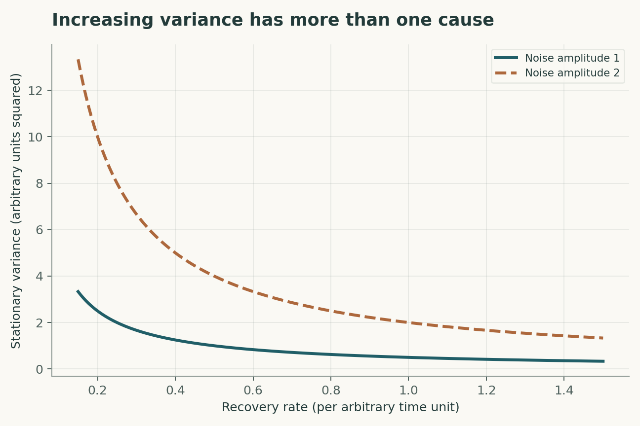
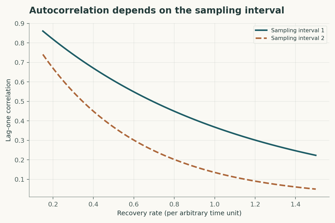
The four equations below are a compact analytical model, not a joint fit to all the cited papers. Their interpretation is as follows. An Ornstein-Uhlenbeck model describes a fluctuation X with positive restoring rate lambda and white-noise amplitude sigma. Stationary variance increases as restoring strength weakens only under the model's stationarity and noise assumptions. Autocorrelation at lag tau increases when lambda decreases; colored forcing can produce alternative behavior. A schematic proxy Y mixes circulation-related X, external forcing F and observation error; coefficients require validation.
The observational target is transport estimates and the restoring dynamics of a specified observable. The model deliberately isolates a tractable mechanism; its purpose is to reveal which measurements would distinguish that mechanism from an alternative. Parameter values in the figures are declared illustrative inputs. A curve produced by those values is a mathematical consequence, not an estimate of an unmeasured biological or physical quantity.
A discriminating validation design
The primary comparison should test early-warning behavior against plausible nonstationary null models. The unit of independent replication is independent time block or observing array; repeated readings from the same unit improve precision but do not create independent replication. A strong validation would hold out other latitudes and historical periods before choosing thresholds or fitting nuisance corrections. In particular, proxy mixing, colored forcing and short observation records must be measured, constrained or varied in a sensitivity analysis. Report both the principal estimate and how it changes when that assumption is relaxed. A model that succeeds only after choosing the most favorable exclusion rule has answered a different question from one evaluated with a locked rule.
Worked numerical analysis
For sigma = 1 in arbitrary units, lambda = 1 gives stationary variance 0.5 and lag-one correlation about 0.368. Reducing lambda to 0.2 gives variance 2.5 and correlation about 0.819. Increasing sigma at fixed lambda increases variance without changing this model's autocorrelation. The paired plots expose this partial distinction, while leaving colored noise and proxy mixing as unresolved alternatives. No collapse date is calculated.
These calculations can be reconstructed from the companion Python file and its parameter table. Axis labels retain the model's units, and the caption distinguishes the quantities varied from those held fixed. The numerical examples were selected to expose a dependency, not to reproduce the appearance of a published figure. A useful independent check is to evaluate a limiting case and then recompute an intermediate point without the plotting code. Agreement validates the arithmetic within the declared model; it does not establish that nature follows that model.
Evidence, transfer and next steps
The scope of the conclusion is limited by proxy mixing, colored forcing and short observation records. Transfer to other latitudes and historical periods requires evidence beyond fitting the original observations. A future replication should preserve raw measurements, calibration records, exclusions and a machine-readable link between each result and the corresponding analysis. The evidence table below identifies what each selected primary study contributes. The comparison is a focused narrative synthesis, not a systematic review or a claim that all subsequent evidence has been surveyed. The proposed study has not been performed here. Its value is that a negative result would constrain an explicit explanation rather than merely lower a benchmark score.
A declared analytical model
Four equations, explicit assumptions
(1) An Ornstein-Uhlenbeck model describes a fluctuation X with positive restoring rate lambda and white-noise amplitude sigma.
(2) Stationary variance increases as restoring strength weakens only under the model's stationarity and noise assumptions.
(3) Autocorrelation at lag tau increases when lambda decreases; colored forcing can produce alternative behavior.
(4) A schematic proxy Y mixes circulation-related X, external forcing F and observation error; coefficients require validation.
Constructed examples · Reproducible data
Inspect the quantitative argument
These curves are calculated from the declared models. They are not observations from the cited studies. Every figure includes its numeric data and vector version.


Which evidence answers which question?
| Evidence or design choice | What it identifies | What remains unresolved |
|---|---|---|
| Source 1 | RAPID methodology estimates overturning at 26 degrees north. | A section estimate is not a direct whole-basin stability measure. |
| Source 2 | OSNAP observations resolved subpolar overturning contributions. | Region and record length differ from subtropical observations. |
| Source 3 | Early-warning analysis examined changing stability indicators. | Indicator interpretation depends on proxy and stochastic assumptions; correction 10.1038/s41558-021-01184-6 fixes a URL. |
| Source 4 | A hydrographic reconstruction found no overall decline over its examined multidecadal interval. | Reconstruction scope does not settle all timescales or future behavior. |
| Primary observable | transport estimates and the restoring dynamics of a specified observable | proxy mixing, colored forcing and short observation records |
| Independent test | early-warning behavior against plausible nonstationary null models | Requires new measurements |
| Transfer set | other latitudes and historical periods | Not validated by the constructed numerical example |
A proposed validation protocol
This is a proposed evaluation design. No new biological experiment, clinical trial or physical experiment was carried out for this article.
- Specify transport estimates and the restoring dynamics of a specified observable before fitting.
- Retain independent identifiers for each independent time block or observing array.
- Separate other latitudes and historical periods from model development.
- Measure or bound proxy mixing, colored forcing and short observation records.
- Record units, calibration and the observation operator.
- Compare the primary model with a named rival explanation.
- Prespecify the test: early-warning behavior against plausible nonstationary null models.
- Archive raw data, exclusions, parameter files and executable analysis.
What the primary sources establish
G.D. McCarthy, D.A. Smeed, W.E. Johns et al. · 2015 [1]
Contribution. RAPID methodology estimates overturning at 26 degrees north.
Boundary. A section estimate is not a direct whole-basin stability measure.
Source locator. Abstract / selected primary-source sections; see linked bibliographic record.
M. S. Lozier, F. Li, S. Bacon et al. · 2019 [2]
Contribution. OSNAP observations resolved subpolar overturning contributions.
Boundary. Region and record length differ from subtropical observations.
Source locator. Abstract / selected primary-source sections; see linked bibliographic record.
Niklas Boers · 2021 [3]
Contribution. Early-warning analysis examined changing stability indicators.
Boundary. Indicator interpretation depends on proxy and stochastic assumptions; correction 10.1038/s41558-021-01184-6 fixes a URL.
Source locator. Abstract / selected primary-source sections; see linked bibliographic record.
Emma L. Worthington, Ben I. Moat, David A. Smeed et al. · 2021 [4]
Contribution. A hydrographic reconstruction found no overall decline over its examined multidecadal interval.
Boundary. Reconstruction scope does not settle all timescales or future behavior.
Source locator. Abstract / selected primary-source sections; see linked bibliographic record.
Limits of this analysis
- A section estimate is not a direct whole-basin stability measure.
- Region and record length differ from subtropical observations.
- Indicator interpretation depends on proxy and stochastic assumptions; correction 10.1038/s41558-021-01184-6 fixes a URL.
- Reconstruction scope does not settle all timescales or future behavior.
- Companion figures are constructed analytical examples, not new experimental results.
- Transfer to other latitudes and historical periods has not been demonstrated by this review.
A focused narrative analysis of the named primary studies, not a systematic literature search or a claim to comprehensive coverage through 2026.
Questions that would change the conclusion
- Which proxy combinations best separate forcing from circulation change?
- How long must direct records be to constrain stability indicators?
- Which nonstationary null models survive cross-array validation?
References
- G.D. McCarthy, D.A. Smeed, W.E. Johns et al.. Measuring the Atlantic Meridional Overturning Circulation at 26°N. Progress in Oceanography (2015). 10.1016/j.pocean.2014.10.006.
- M. S. Lozier, F. Li, S. Bacon et al.. A sea change in our view of overturning in the subpolar North Atlantic. Science (2019). 10.1126/science.aau6592.
- Niklas Boers. Observation-based early-warning signals for a collapse of the Atlantic Meridional Overturning Circulation. Nature Climate Change (2021). 10.1038/s41558-021-01097-4.
- Emma L. Worthington, Ben I. Moat, David A. Smeed et al.. A 30-year reconstruction of the Atlantic meridional overturning circulation shows no decline. Ocean Science (2021). 10.5194/os-17-285-2021.
The publisher correction repairs the data-access URL. It is retained here to keep the source and its accessible data record connected. Publisher update.
Bibliographic identity checked against Crossref. Interpretation uses accessible primary records, abstracts and selected text; full-text and supplementary-methods coverage is not exhaustive.
Authorship and provenance
Source-based research review and original mathematical analysis written by Codex (AI). Cited experiments belong to the cited research teams.
Concept cover created with the built-in ImageGen tool. Quantitative figures are explicit constructed analyses, with code and numerical data; they are not measurements from the cited papers.
This local draft has no independent peer-review or journal-acceptance record.