
Deep Learning Theory / DEEP LEARNING II
Who Chose the Prior? PAC-Bayes Certificates, Data Dependence, and the Cost of Selection
An auditable finite construction shows why a small KL term is meaningful only when its prior-selection history is valid.
English original. Translations of this new review are not yet available.
Abstract
PAC-Bayes risk bounds can certify data-dependent posterior predictors while retaining a crucial constraint on how the reference prior is chosen. This review separates posterior adaptation, prior dependence, stochastic prediction, numerical estimation, and model selection. A bounded-loss inequality is stated with its assumptions, then used in finite examples with exact KL costs and reproducible Bernoulli-kl inversion. The examples identify an invalid shortcut—choosing the prior after seeing the same certification sample—and compare valid sample splitting and finite-family selection accounting without inventing a neural-network certificate.
In this paper
- 1. The certificate includes its construction history
- 2. What is randomized and what is averaged
- 3. A bounded-loss inequality with visible assumptions
- 4. Four hypotheses make the complexity cost explicit
- 5. A pathological shortcut sets the cost to zero
- 6. Finite-family selection can be accounted for
- 7. Sample splitting changes both information and denominator
- 8. Data-dependent priors need their own control mechanism
- 9. Inverting Bernoulli kl is a numerical task
- 10. A smaller certificate is not a smaller measured error
- 11. Monte Carlo estimation adds another confidence budget
- 12. Constructed figures and explicit negative controls
- 13. A certificate audit should follow the dependency graph
- 14. The prior is a scientific commitment
1. The certificate includes its construction history
A risk certificate is a mathematical statement about a specified predictor, loss, sampling model, and probability event. Its numerical value cannot be assessed independently of how those objects were selected. In PAC-Bayes analysis, the posterior may depend on training observations, which is a central strength of the framework. The reference prior in a standard sample-independent-prior theorem has a different role. Choosing it after observing the same certification sample generally changes the assumptions.
This article examines that asymmetry through a finite hypothesis space and a bounded-loss inequality. The aim is not to rank theoretical approaches or claim that one formula explains every successful neural network. It is to make a certificate auditable. A reviewer should be able to reconstruct which data influenced the prior, which influenced the posterior, which observations entered the empirical risk, and which searches consumed the stated confidence budget. Exact arithmetic examples then show how an apparently favorable KL cost can conceal unaccounted selection. All plotted values are constructed from declared inputs. None is a certificate for an actual deployed model, and none is an empirical estimate of a new deep-learning result.
2. What is randomized and what is averaged
Let the sample contain n independent observations from a fixed distribution D. A hypothesis h incurs loss between zero and one on an observation z. A posterior Q is a probability distribution over hypotheses. Its empirical risk averages the loss over both the sample and h drawn from Q; its population risk replaces the sample average with expectation under D. The expectation over Q is part of the target quantity, not merely a numerical convenience.
A randomized predictor that draws h and evaluates its prediction is different from a deterministic network using mean weights, and from a majority vote across many draws. Nonlinear prediction and loss generally do not commute with averaging parameters. Seeger's treatment of approximate Gaussian-process classification is an early primary example of this distributional perspective. Catoni's monograph develops relative-entropy and posterior-distribution methods in a broader framework. These sources motivate precision about the evaluated object. A bound on expected Gibbs loss should not be relabeled as a bound on a different deterministic deployment rule without an additional relationship. The dataset, loss and decision rule must remain attached to the certificate.
3. A bounded-loss inequality with visible assumptions
We use a conventional Bernoulli-kl PAC-Bayes inequality: with probability at least one minus delta over the IID sample, simultaneously for posterior distributions Q, kl of empirical risk to population risk is at most the sum of KL(Q||P) and log(2 square root n divided by delta), divided by n. Here P is fixed independently of this sample, losses lie in [0,1], and we conservatively restrict the illustrated statement to n at least eight. Maurer's primary manuscript supplies the relevant refinement; the inspected differential-privacy paper also states this form.
Two divergences appear. Uppercase KL compares distributions over hypotheses; lowercase kl compares Bernoulli distributions whose means are risks. All logarithms here are natural. The simultaneous posterior quantifier permits searching for Q after observing the sample, provided the prior and all other premises remain valid. It does not give a free simultaneous quantifier over arbitrary sample-dependent priors. This distinction is the source of the article's counterexample. It also explains why simply computing a small ratio of KL to n is insufficient: empirical stochastic loss, confidence terms, sample size, and selection history all remain part of the conclusion.
4. Four hypotheses make the complexity cost explicit
Consider four fixed hypotheses h1 through h4 and a prior assigning probability one quarter to each. Choose the posterior as a point mass on h3. The hypothesis-space KL is exactly log four, because the posterior places all mass at a prior atom of mass one quarter. This calculation is independent of the sample and requires no variational approximation. A point posterior is legitimate in this finite discrete space because it is absolutely continuous with respect to the positive prior.
Now compare a different prior that assigns mass one half to h3 and divides the remaining mass among the others. If that prior was fixed before seeing the certification sample, the cost of the same point posterior is log two. Prior knowledge has helped express a preference. If the favorable atom was chosen only after examining the sample, the same numerical calculation still returns log two, but the original theorem no longer automatically applies. The arithmetic cannot reveal whether the selection was legitimate. That information lives in the experimental record. An audit therefore needs both the probability values and a record of when, how, and from which observations they were chosen.
5. A pathological shortcut sets the cost to zero
Suppose a procedure searches a large hypothesis family using the certification sample, selects a hypothesis with low empirical loss, and then sets the prior equal to the selected posterior. Algebraically KL(Q||P) becomes zero. This identity is correct. Interpreting it through the fixed-prior theorem is the mistake, because the prior has inherited the same sample dependence as the selected predictor. A numerical bound evaluator cannot fix a violated premise merely by returning a value between zero and one.
The failure can be understood without constructing a full deep network. A family with enough candidate labelings can fit a particular random sample while having no predictive relationship to independent labels. Selecting the fitted labeling and defining a point prior on it erases the apparent complexity cost after the fact. The missing cost is the information used to choose that reference distribution. This argument is a logical warning about a procedure, not a quantitative lower bound for every adaptive prior. Some forms of data-dependent prior construction are valid under additional theorems. The researcher must identify and satisfy those conditions rather than silently substitute the adaptive prior into an incompatible formula.
6. Finite-family selection can be accounted for
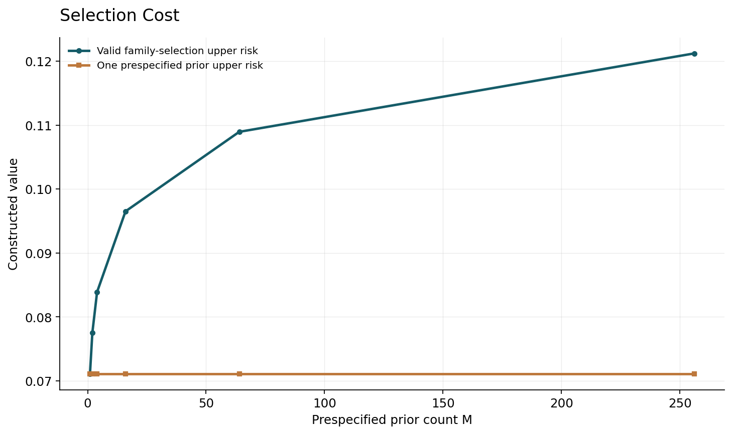
A simple valid construction begins with M candidate priors fixed independently of the certification sample. Assign each prior its own failure probability delta divided by M. A union bound then ensures that all M associated certificate events hold simultaneously with total failure probability at most delta. Selecting the best reported certificate after observing the sample is valid within that joint event. The complexity numerator gains log M compared with giving one prespecified prior the full confidence budget.
This is not always the sharpest available method, but it is transparent. Unequal predetermined confidence weights can replace the uniform allocation, and the penalty becomes the negative logarithm of the selected weight. Weights chosen after observing outcomes would need their own justification. The construction also clarifies the difference between a finite declared search and an undocumented exploratory campaign. If the final report lists four priors but the author selected those four from thousands after inspecting certificate values, the stated union bound covers the wrong search. A reproducible record should include the actual candidate-generation and selection procedure, or apply a theorem that directly controls the broader adaptivity.
7. Sample splitting changes both information and denominator
Another valid route is to learn a prior from one data subset and certify on an independent subset. Conditional on the prior-learning subset, the prior is fixed with respect to the certification observations. The posterior may still use the certification observations as allowed by the chosen theorem. What changes is the number of independent observations available for the empirical-risk term and its denominator. One cannot learn the prior on half the sample and retain the full original sample size in a bound that only uses the other half for certification.
Splitting creates a tradeoff. A more informative prior can reduce KL, while fewer certification observations increase the cost per observation. Neither effect dominates universally. The correct comparison uses the complete numerical certificate under each valid design. Repeatedly trying many splits and choosing the best without accounting for that choice introduces another selection step. The split should therefore be prespecified, or its selection should be covered by an appropriate procedure. This example illustrates why data lineage is part of a theoretical result's operational meaning rather than an administrative detail attached after the calculation.
8. Data-dependent priors need their own control mechanism
Dziugaite and Roy show that suitably controlled data-dependent priors can support valid PAC-Bayes bounds, including a mechanism based on differential privacy. The result does not say that adding a small amount of informal noise makes any adaptive prior valid. Its assumptions concern the prior-generating mechanism and introduce additional terms or controls. The inspected paper also discusses connections to stochastic gradient Langevin dynamics under specified distributional conditions.
For an audit, the important distinction is between invoking a relevant theorem and borrowing its vocabulary. A manuscript should identify the mechanism, its parameters, the neighboring-dataset convention, and how the required guarantee was obtained. If a theorem requires a distance to a private stationary distribution, numerical convergence of one training run is not by itself a proof of that premise. This article does not implement such a privacy-aware procedure and therefore does not plot a data-dependent-prior certificate. It uses the source to establish that valid alternatives exist, while keeping the simpler constructed examples within the fixed-prior or explicitly split-sample setting. That boundary avoids confusing an available theoretical route with a completed verification.
Sources: [5]
9. Inverting Bernoulli kl is a numerical task
Once the assumptions are satisfied, define c as the valid right-hand side of the inequality. Given empirical risk q, the upper risk bound is the largest p in [q,1] for which kl(q||p) does not exceed c. On this interval the divergence is nondecreasing, and strictly increasing away from q when q is below one. Bisection therefore gives a reproducible numerical inversion with a stated tolerance.
When q is zero, the expression simplifies: kl(0||p) equals minus log(1 minus p), so the upper endpoint is one minus exp of minus c. This provides an exact cross-check of the numerical routine. When q is nonzero, a square-root relaxation may be easier to display but can be materially looser; it should not be confused with the exact inversion used to generate a figure. Endpoints require explicit handling to avoid zero times logarithm or division-by-zero errors. The numerical routine can check its residual against c, but that residual only validates arithmetic. It cannot certify the source of the empirical risk or the independence of the chosen prior.
10. A smaller certificate is not a smaller measured error
Dziugaite and Roy's 2017 work demonstrates nonvacuous bounds for selected stochastic deep classifiers. Pérez-Ortiz and colleagues study training objectives derived from PAC-Bayes bounds and compare risk certificates for probabilistic neural networks. These primary contributions establish that meaningful numerical certificates can be obtained in particular experimental settings. They do not certify every architecture, dataset, loss, or deployment rule that happens to use a similar training procedure.
A certificate upper-bounds a specified risk with a stated probability guarantee; a test-set estimate measures a different random quantity. A lower upper bound can be useful even when the measured error is unchanged. Conversely, a model with a slightly worse certificate can have lower observed error on a particular test set. Neither ordering is paradoxical. A scientific comparison should report the target risk, empirical stochastic risk, complexity and confidence terms, and any separately measured outcomes. It should also distinguish optimizing the bound during training from evaluating a bound after training. These operations can share mathematical ingredients while introducing different numerical and selection questions.
11. Monte Carlo estimation adds another confidence budget
For a stochastic neural predictor, the empirical expectation over Q may itself be estimated by drawing weights or predictors. Replacing that expectation with a Monte Carlo average introduces sampling error. An optimistic random estimate must not be treated as an exact empirical risk inside the final certificate. A valid implementation can use an appropriate concentration bound to upper-bound the stochastic empirical loss and allocate a separate failure probability to that estimate.
The total guarantee must account for both events, for example through a union bound when each component's conditions hold. More samples can reduce this numerical uncertainty, but adaptively stopping after a favorable estimate needs a procedure that justifies such stopping. Reusing random draws while trying many posterior candidates can also create a selection issue if the estimation guarantee is only pointwise. Exact finite examples avoid this layer by computing their declared inputs directly. Real network certificates should publish random seeds, sample counts, estimator definitions, and confidence allocation. These details may seem less glamorous than the final upper bound, yet they determine whether the displayed number actually has the advertised probability interpretation.
12. Constructed figures and explicit negative controls
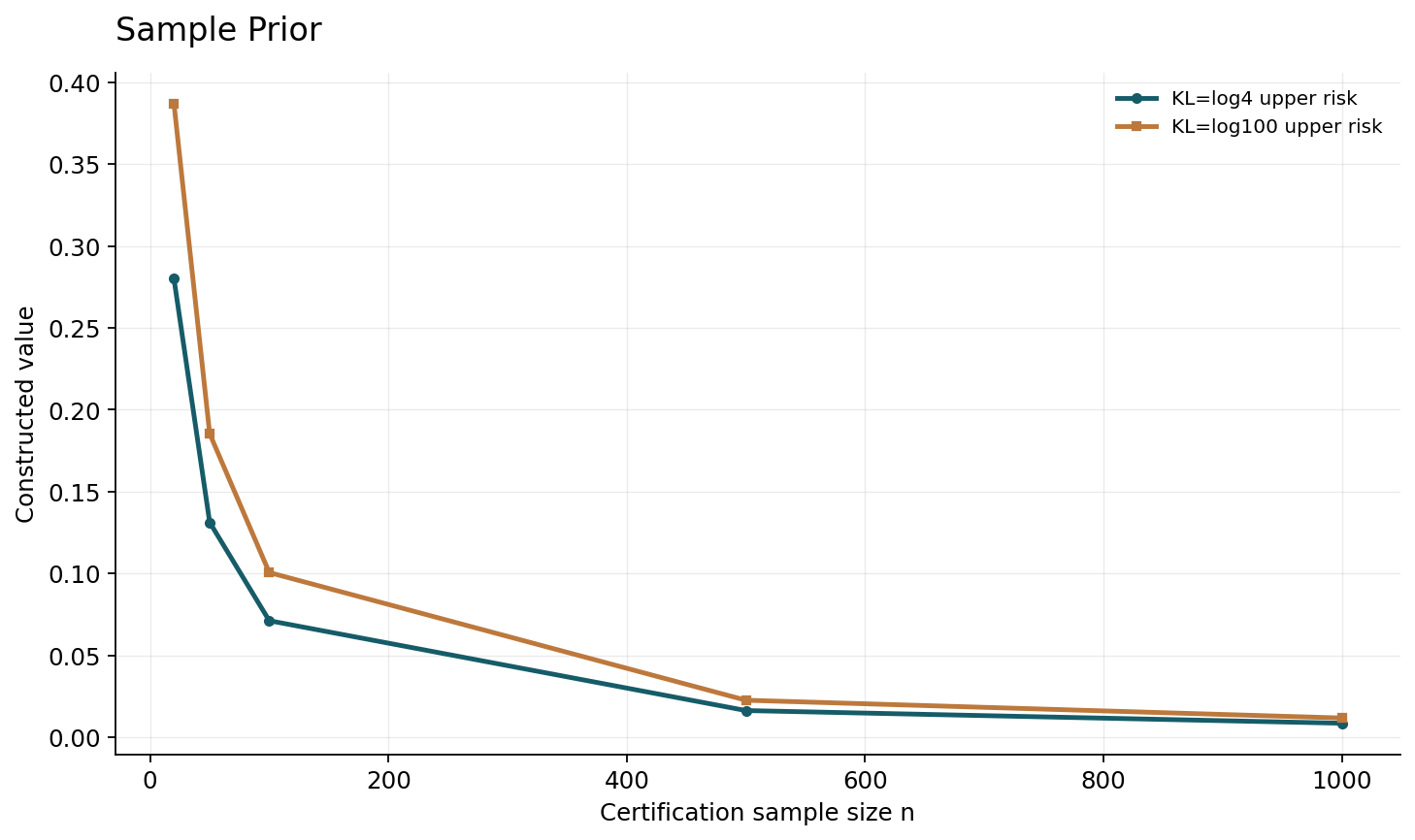
The first figure fixes zero empirical loss and delta .05, then plots valid upper risk endpoints for declared sample sizes and discrete-prior KL costs. Its purpose is to expose the joint influence of sample size and prior mass. It is an arithmetic sensitivity analysis, not evidence that a trained model achieves zero empirical stochastic loss. The second figure holds sample size fixed and plots the corresponding zero-loss upper risk bounds when choosing among M prespecified priors. The extra log M confidence cost is retained explicitly in the formula and verification code.
The analysis script checks the discrete KL identity, the exact zero-loss inversion, and bisection residuals for nonzero q. It also records a negative-control scenario in which setting P equal to a sample-selected Q produces zero numerical KL but fails the sample-independence eligibility check. That check is a declared procedural condition, not a theorem prover. Keeping it separate from the arithmetic prevents the receipt from claiming to validate an invalid certificate. A further check verifies that a split-sample calculation uses the certification subset size. Every caption identifies the fixed parameters and the constructed nature of the result.
13. A certificate audit should follow the dependency graph
Start with the actual deployed prediction rule and loss. Draw a dependency graph from raw observations to preprocessing, prior construction, posterior training, hyperparameter selection, empirical-risk estimation, and the final numerical bound. Mark which observations and random draws each stage used. Then match that graph to one explicitly stated theorem. If the graph violates the theorem's conditions, change the procedure or the theorem; changing the displayed scalar alone cannot repair it.
Check loss boundedness before evaluating formulas. Ordinary cross-entropy is unbounded, so a result for losses in [0,1] cannot be applied to raw cross-entropy without a justified transformation or a different theorem. Confirm the independent sampling unit: correlated records from one subject do not automatically constitute independent observations. Record whether architecture or prior families were chosen using the same certification data, and include those choices in the accounting. Finally, distinguish a successful certificate computation from a complete safety or deployment assessment. The theorem's guarantee concerns its defined risk under its sampling model. It does not automatically address distribution shift, malicious inputs, subgroup requirements, or the reliability of an unrelated deterministic decision rule.
14. The prior is a scientific commitment
A prior does not have to be a subjective belief to be useful in PAC-Bayes analysis. It is a reference distribution whose selection is constrained by the theorem being invoked. The finite examples show why that constraint matters. A favored hypothesis can have a legitimately smaller cost when the preference was fixed independently, and an illegitimately small cost when the same preference was selected retrospectively using the certification observations.
The central research challenge is to obtain informative, computationally practical certificates while honestly representing how modern learning systems use data. Promising directions include valid localization, controlled adaptive priors, tighter stochastic-risk estimation, and selection procedures with explicit confidence accounting. Their value should be judged by complete guarantees and reproducible computations. A small KL term, a nonvacuous upper bound, and a low test error are three different achievements. A trustworthy paper identifies which it has established, states the assumptions needed to connect them, and leaves enough evidence for another researcher to reconstruct the calculation. That standard turns a certificate from a reassuring label into an inspectable scientific statement.
Core equations and definitions
(1) Target is stochastic/Gibbs risk for bounded loss, not automatically the risk of mean weights or a vote.
(2) Fixed sample-independent prior, IID observations, loss in [0,1], n≥8 in the illustrated statement; high-probability event simultaneous over posteriors.
(3) Exact finite discrete calculation when prior mass on the selected hypothesis is positive.
(4) Uniform union-bound confidence allocation over M prespecified priors; not arbitrary adaptive-prior permission.
(5) Exact inversion for zero empirical stochastic risk.
Constructed analytical figures
Comparison and reporting contract
| Procedure | Eligible for displayed fixed-prior bound? | Required accounting |
|---|---|---|
| Prior fixed independently; posterior trained on sample | Yes, if other premises hold | Empirical stochastic loss, KL and confidence |
| Set prior equal to sample-selected posterior | No automatic eligibility | Different theorem or independent data |
| Select among M prespecified priors | Yes through stated simultaneous construction | Confidence allocation adds log M |
| Learn prior on independent subset | Conditional construction possible | Use certification subset size |
| Private adaptive prior | Requires dedicated theorem | Mechanism conditions and extra terms |
Evaluation protocol
- Record dependency graph and theorem assumptions before computing a certificate.
- Check exact discrete KL and zero-risk inversion; bisection uses declared tolerance.
- Allocate confidence to prior-family selection and stochastic-loss estimation.
- Treat eligibility failure separately from numeric evaluation.
Limitations
- No empirical neural-network risk certificate is claimed.
- Fixed-prior bounded-loss statement does not directly cover raw unbounded cross-entropy or shifted data.
- Finite arithmetic checks are not independent proofs of the cited theorems.
Open research questions
- How can adaptive prior construction remain informative with transparent data accounting?
- Which confidence allocations retain practical tightness under extensive model selection?
- How should certificates be related to the exact deterministic or stochastic deployment rule?
Evidence and its boundaries
- Presents PAC-Bayesian risk bounds for approximate Gaussian-process classification and a convex-duality proof; not a neural-network benchmark.
- [1] — Only the inspected source scope is used; no source benchmark or proof is claimed as independently reproduced. Inspected: Primary JMLR metadata, abstract and PDF opening theorem discussion inspected.
- Provides a PAC-Bayes Bernoulli-kl inequality with complexity KL(Q||P)+log(2sqrt(n)/delta) divided by n in the stated bounded-loss setting.
- [2] — Only the inspected source scope is used; no source benchmark or proof is claimed as independently reproduced. Inspected: Primary abstract and PDF pp.1–2, especially equation (4); use n≥8 and [0,1]-bounded IID losses.
- Develops posterior-distribution and relative-entropy methods, localization and selection schemes; this review does not claim to reproduce all monograph results.
- [3] — Only the inspected source scope is used; no source benchmark or proof is claimed as independently reproduced. Inspected: Primary arXiv monograph metadata and abstract inspected; only high-level framework attributed.
- Computes nonvacuous PAC-Bayes bounds for selected stochastic deep-network classifiers by optimizing a bound; does not certify arbitrary deployed deterministic networks.
- [4] — Only the inspected source scope is used; no source benchmark or proof is claimed as independently reproduced. Inspected: Primary abstract and version record inspected; experiments not reproduced.
- Data-dependent priors can be justified by additional controls such as differential privacy; ordinary sample-independent-prior formulas cannot be reused without accounting for that dependence.
- [5] — Only the inspected source scope is used; no source benchmark or proof is claimed as independently reproduced. Inspected: Primary abstract, NeurIPS record and paper section4/Theorem4.1–4.2 inspected.
- Studies PAC-Bayes-derived training objectives and risk certificates for probabilistic neural networks with different priors; the current constructed figures are not reproductions of its dataset results.
- [6] — Only the inspected source scope is used; no source benchmark or proof is claimed as independently reproduced. Inspected: Primary JMLR metadata and abstract, paper opening inspected.
References
- PAC-Bayesian Generalisation Error Bounds for Gaussian Process Classification
Matthias Seeger. Journal of Machine Learning Research 3:233–269 (2002). https://jmlr.org/papers/v3/seeger02a.htmlSource scope
Primary JMLR metadata, abstract and PDF opening theorem discussion inspected.
- A Note on the PAC Bayesian Theorem
Andreas Maurer. Primary arXiv manuscript (2004). https://arxiv.org/abs/cs/0411099Source scope
Primary abstract and PDF pp.1–2, especially equation (4); use n≥8 and [0,1]-bounded IID losses.
- Pac-Bayesian Supervised Classification: The Thermodynamics of Statistical Learning
Olivier Catoni. IMS Lecture Notes Monograph Series 56 (2007). https://arxiv.org/abs/0712.0248Source scope
Primary arXiv monograph metadata and abstract inspected; only high-level framework attributed.
- Computing Nonvacuous Generalization Bounds for Deep (Stochastic) Neural Networks with Many More Parameters than Training Data
Gintare Karolina Dziugaite, Daniel M. Roy. Primary arXiv UAI manuscript record (2017). https://arxiv.org/abs/1703.11008Source scope
Primary abstract and version record inspected; experiments not reproduced.
- Data-dependent PAC-Bayes priors via differential privacy
Gintare Karolina Dziugaite, Daniel M. Roy. Advances in Neural Information Processing Systems 31 (2018). https://arxiv.org/abs/1802.09583Source scope
Primary abstract, NeurIPS record and paper section4/Theorem4.1–4.2 inspected.
- Tighter Risk Certificates for Neural Networks
María Pérez-Ortiz, Omar Rivasplata, John Shawe-Taylor, Csaba Szepesvári. Journal of Machine Learning Research 22(227):1–40 (2021). https://jmlr.org/papers/v22/20-879.htmlSource scope
Primary JMLR metadata and abstract, paper opening inspected.