
Deep Learning Representations / DEEP LEARNING II
Learning from a Moving Teacher: Self-Distillation, Temporal Smoothing, and Collapse Boundaries
A finite exponential-average model reveals the variance–lag tradeoff while a constant-map counterexample limits what consistency alone can promise.
English original. Translations of this new review are not yet available.
Abstract
Self-distillation combines several distinct mechanisms: transferring soft predictions, averaging a teacher over time, asymmetric gradients, and learning representations from paired views. This analytical review separates those mechanisms using primary papers and exact scalar constructions. Exponential averaging yields explicit weights, a stationary-noise variance and a lag under drift, while nonlinear weight averaging and a constant-map consistency solution expose important boundaries. Reproducible calculations support a controlled evaluation protocol without presenting temporal smoothing as a proof that a self-supervised neural system avoids collapse or improves downstream accuracy.
In this paper
- 1. A teacher is a mechanism, not an extra source of truth
- 2. Same capacity does not imply the same training problem
- 3. Soft targets change the gradient direction
- 4. Weight averages and output averages are different
- 5. Unrolling a scalar moving teacher
- 6. Stationary noise reduction has strict assumptions
- 7. Smoothing introduces lag under drift
- 8. Consistency admits an uninformative zero-loss map
- 9. Successful paired-view methods are complete procedures
- 10. Stop-gradient changes dynamics without changing a value
- 11. A theoretical mechanism needs its data model
- 12. A finite verification and figure specification
- 13. An empirical study should test the whole learning claim
- 14. Better teachers require more than slower movement
1. A teacher is a mechanism, not an extra source of truth
A student trained from a teacher can behave differently even when both use the same architecture and underlying observations. The target distribution, optimization path, augmentation, training budget and selection rule can all change. Saying that the student learns from itself groups these effects under one phrase, but does not explain which effect produced an improvement. A useful analysis separates what information is reused from how the procedure processes it.
This article focuses on teacher dynamics and their boundaries. We distinguish sequential same-architecture distillation, moving-average teachers, paired-view consistency and asymmetric gradient updates. Selected primary studies establish that these designs have produced useful results in specified settings. An exact scalar exponential average then exposes a tradeoff between noise reduction and delayed tracking. A constant-representation construction shows why a small consistency objective alone does not guarantee useful features. The calculations are not simulations of a full neural training method and do not reproduce reported downstream accuracies. Their purpose is to identify which claims follow from a stated recurrence, which depend on architectural and optimization choices, and which require an independent empirical evaluation of the learned representation.
2. Same capacity does not imply the same training problem
Furlanello and colleagues study born-again networks, where students can have the same parameterization as their teachers. Their experiments demonstrate that distillation need not be limited to compressing a larger model into a smaller one. A student can receive a different training signal from a teacher's distribution over outputs even when both networks have equal nominal capacity. This is an empirical result within the tested procedures, not a guarantee that another generation always helps.
The comparison should retain the full cost of training the teacher and student, and should state whether performance is measured for one student or an ensemble of generations. Additional training and repeated selection can themselves improve outcomes. A clean study includes a matched-budget baseline that continues or restarts ordinary training under a comparable schedule. It also preserves the labels and observations actually available to each method. The teacher does not supply an independently verified new label merely because its output is softer than the original target. Distillation transforms and reweights information through a learning procedure. Whether that transformation improves prediction is a testable outcome rather than an implication of equal architecture or a persuasive teaching metaphor.
Sources: [1]
3. Soft targets change the gradient direction
For a categorical student distribution p obtained from logits and a fixed teacher distribution q, cross-entropy with q has logit gradient p minus q at unit temperature. Training with a one-hot label instead gives p minus the one-hot vector. The teacher can therefore redistribute the gradient across classes, including classes that are not its highest-scoring prediction. Matching only its hard decision discards that distributional structure.
This identity explains a mechanism but does not establish that every teacher distribution is helpful. A confidently wrong teacher can reinforce an error, and a teacher trained with a biased data source can transmit that bias. Temperature scaling changes both target softness and gradient scale, so a fair experiment records the exact objective, temperature factors and weighting against labeled loss. The teacher's nonwinning probabilities should not be described as inherently correct semantic knowledge without further evidence. They are model outputs. A useful ablation can compare full distributions, hard pseudo-labels and controlled transformations of the nonwinning probabilities while keeping compute and selection comparable. The result can identify which signal matters in a tested procedure without proving a universal theory of information transfer.
4. Weight averages and output averages are different
Tarvainen and Valpola's Mean Teacher uses moving averages of model weights for consistency targets, distinguishing it from averaging predictions for individual examples. For a nonlinear network, the prediction at averaged parameters generally differs from the average prediction. This distinction is essential before applying a scalar filtering calculation to a neural teacher.
An exact counterexample uses f_theta=theta squared. Two parameter values minus one and plus one each give output one. Their mean parameter is zero and gives output zero, while their mean output remains one. Thus a claim about noise variance in a scalar average of predictions is not automatically a claim about a weight-averaged nonlinear model. A local linearization may sometimes motivate an approximation, but it needs an error assessment and a declared regime. The calculations below deliberately analyze a scalar sequence s_t and its exponential average q_t. They can describe a coordinate average exactly, or an output average if that is what s_t denotes. They do not identify these two interpretations. A network study should report which object is averaged and how normalization buffers or other nonparameter state are handled.
Sources: [2]
5. Unrolling a scalar moving teacher
Let q_t equal beta times q_(t minus one) plus one minus beta times s_t, with beta between zero and one and an explicit initial q_0. Repeated substitution yields beta to the t times q_0 plus a weighted sum of past s values. The newest value has weight one minus beta, the next has weight beta times one minus beta, and each additional delay introduces another factor beta. The observed weights sum to one minus beta to the t; the initial state carries the remaining mass.
Initialization therefore matters at finite time. Starting from zero creates a different early target from starting at the first student value. Dividing by one minus beta to the t gives a particular bias-corrected estimator when a zero initialization is intended, but it is a changed recurrence output and should be reported. For beta close to one, the initial contribution can persist for many steps. A schedule that changes beta also changes the kernel: the simple geometric formula no longer applies unchanged. The finite verification script checks the recurrence against its unrolled form, including initial mass. This arithmetic is useful for understanding target history without claiming that one smoothing coefficient is optimal for every learning problem.
6. Stationary noise reduction has strict assumptions
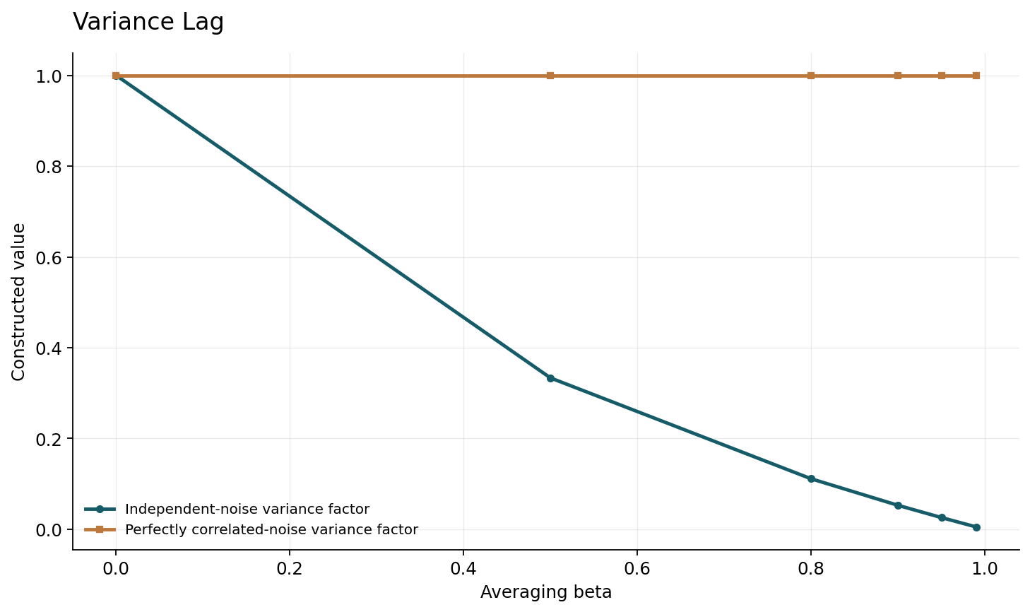
Suppose s_t equals a constant signal m plus independent zero-mean noise with variance sigma squared, and consider the infinite-history stationary exponential average. Summing squared geometric weights gives variance sigma squared times (one minus beta) divided by (one plus beta). The equivalent independent-sample count under this specific variance comparison is (one plus beta) divided by (one minus beta). It grows as beta approaches one.
This is not the number of independent neural models represented by a moving teacher. Successive training checkpoints are correlated, the signal changes during optimization, and different parameter directions can have different noise structure. Positive temporal correlation introduces covariance terms that the independent-noise formula omits. The variance identity should therefore be used as a baseline with visible assumptions. In a real experiment, estimate relevant autocorrelations or compare directly against observed target variability, and retain the limitations of that estimate. A smoother output can also be smoothly wrong. Noise reduction in a chosen coordinate is an arithmetic property, while better downstream prediction is a separate outcome requiring labels or other task-specific evidence. The construction deliberately keeps those claims separate.
7. Smoothing introduces lag under drift
Now let the scalar signal increase linearly as m_t=v times t, with a teacher that has reached the corresponding steady tracking regime. The average delay of the infinite geometric kernel is beta divided by one minus beta. The expected teacher value therefore trails the current signal by v times that delay. Increasing beta lowers stationary independent-noise variance but increases lag under this declared drift model.
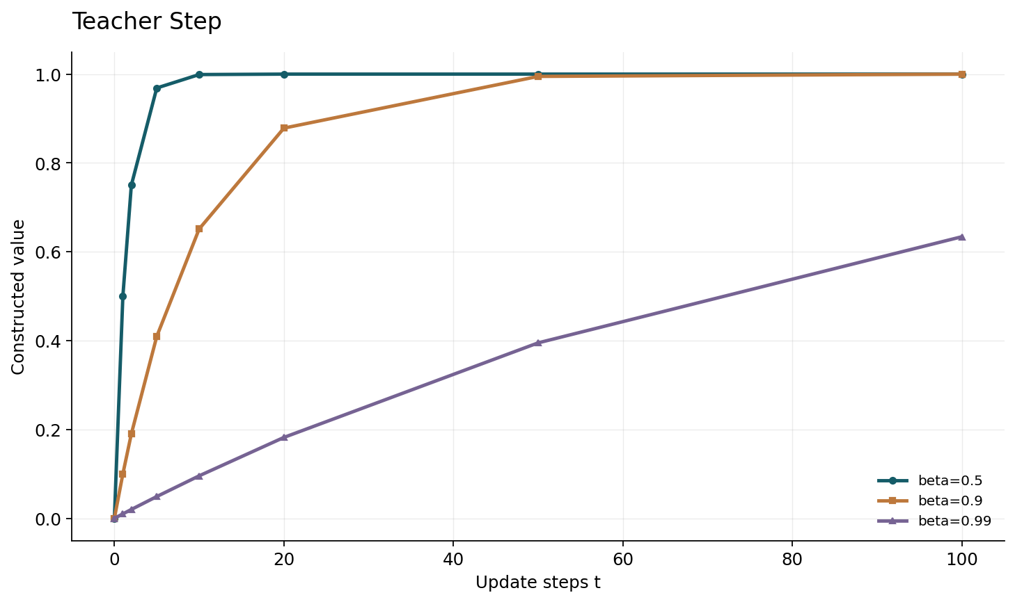
The tradeoff is visible without inventing an empirical performance curve. For beta .9 the mean delay is nine steps; for beta .99 it is ninety-nine. These numbers refer to the recurrence's update unit, which might be batches or optimizer steps in an implementation. They are not dataset-independent recommendations. If the underlying signal changes abruptly, finite-time step response gives another useful diagnostic: after a switch from zero to one with initial teacher zero, the output is one minus beta to the t. Both calculations show why a teacher that looks stable can respond slowly to genuine learning. A real schedule may deliberately balance those effects, but its success must be measured under the actual dynamics rather than inferred from a stationary averaging analogy.
8. Consistency admits an uninformative zero-loss map
Consider the naive objective that averages the squared distance between representations of two views of the same observation. A representation g that maps every possible view of every observation to the same constant vector has loss zero. If normalized outputs are required, choose the same nonzero unit vector everywhere; the pairwise agreement remains exact. The representation need not preserve any information that distinguishes observations or labels.
This is an existence counterexample, not a claim that every training run converges to that solution. It establishes that the consistency objective alone does not exclude collapse. Adding an exponential teacher average does not remove the constant solution: if both student and teacher are constant, the average stays constant. Whether a complete algorithm avoids collapse can depend on asymmetric gradients, predictor structure, normalization, centering, objective details and optimization dynamics. Those ingredients must be studied in the actual procedure. A low consistency loss should therefore be accompanied by representation diagnostics such as variance, effective rank and independent downstream evaluation. None of those diagnostics alone proves universal usefulness, but they can falsify the most obvious degenerate explanation for apparent training success.
9. Successful paired-view methods are complete procedures
Grill and colleagues' BYOL couples online and target networks while updating the target through a slow-moving average. Caron and colleagues' DINO interprets a particular vision-transformer procedure as label-free self-distillation and examines a combination of momentum encoder, crops and architectural choices. These studies provide evidence for their complete designs and evaluated protocols. Their results should not be attributed to an arbitrary moving average in isolation.
This distinction guides ablation design. Removing one component can alter both optimization and target statistics, so a failure does not automatically identify a unique causal explanation. Compare changes under matched budgets, document failed runs, and inspect collapse as well as downstream quality. If a modified procedure requires a new learning-rate or temperature schedule, report whether the comparison includes that tuning cost. The scalar construction here isolates smoothing exactly but omits most neural ingredients. It can falsify the claim that averaging alone mathematically excludes constant representations. It cannot determine why BYOL or DINO avoids collapse in a particular implementation, and it cannot rank their transfer quality from an exponential kernel's variance formula.
10. Stop-gradient changes dynamics without changing a value
Chen and He's SimSiam study reports useful representations without requiring a momentum encoder and identifies a stop-gradient operation as important in the tested procedure. This observation limits an overly broad explanation that a slow teacher is necessary for every successful noncontrastive paired-view method. The update rule matters, including which paths receive derivatives, even when the displayed scalar objective appears symmetric.
A stopped-gradient target can have the same numerical value as a differentiable target while producing a different parameter update. One must therefore specify a computational graph, not merely an algebraic loss expression, to describe the learning algorithm. The existence of a collapsed solution and the dynamics near that solution are also distinct questions. An objective can admit a degenerate optimum that a particular asymmetric procedure does not reach under studied conditions. Conversely, observing noncollapse in a few runs is not a proof that all initializations and data distributions avoid it. A reproducible report preserves the exact gradient boundaries and target-update order, and tests both representation quality and stability across the declared training regime.
Sources: [5]
11. A theoretical mechanism needs its data model
Allen-Zhu and Li develop a theoretical account of ensemble, distillation and self-distillation under a specified multi-view data structure. Such work offers a mechanism explaining how different learned views can be combined and transferred in its model. It does not justify asserting the same guarantee for an arbitrary dataset merely because the training procedure contains a teacher and student.
The productive next step is to identify observable implications of the proposed mechanism. Are independently trained teachers using complementary information? Does the student retain that information under controlled probes? Does an ensemble benefit exceed what a matched-budget single model achieves? These questions require an evaluation design that distinguishes representation complementarity from extra compute, augmentation or selection. The scalar averaging model has no multi-view semantics and makes no claim to reproduce that theory. It describes temporal weighting and a collapse boundary. Keeping the models separate allows each to contribute a precise statement without creating a misleading composite theorem. A serious synthesis should state which assumptions would be needed to connect them and which of those assumptions are actually tested in the application.
Sources: [6]
12. A finite verification and figure specification
The supplied script checks recurrence unrolling for several beta values and finite sequences, including a nonzero initial state. It sums sufficiently many geometric weights to verify the stationary-noise variance identity to a declared truncation tolerance. It verifies the first moment of the delay kernel and compares the step response against one minus beta to the t. These calculations use deterministic sums; no Monte Carlo run is presented as a neural benchmark.
The first scientific figure plots exact step responses for beta .5, .9 and .99. The second compares stationary variance factors for independent temporal noise and perfectly shared noise over a declared beta grid. Mean delays are printed separately in the verification output, keeping delay units off the variance axis and avoiding an invented performance score. The script also checks the nonlinear weight-average counterexample and the zero-loss constant-map example. A negative control introduces perfectly correlated scalar noise: averaging does not reduce its variance, demonstrating a boundary of the independent-noise formula. The receipt records the model and checks. It does not certify noncollapse, generalization, or any cited method's implementation, and its labels explicitly preserve that limitation.
13. An empirical study should test the whole learning claim
Define whether the objective is supervised distillation, semi-supervised consistency or self-supervised representation learning. Freeze the data access, teacher source, architecture, augmentations, gradient graph, averaging schedule and selection rule. Compare against matched total compute and matched data rather than only matched student epochs. Evaluate the actual deployment object: student, teacher, ensemble or frozen representation with a declared probe.
Track more than training agreement. Record representation variance and rank, task performance on independent labels, sensitivity to target staleness, and failure rates across seeds. If a downstream linear probe is used, preserve its training and model-selection protocol; a favorable probe is not a direct guarantee for every downstream task. Inspect shifts where the teacher's errors may be shared by the student. Report generations that fail to improve, since repeated selection can otherwise make a sequence of students look consistently better. Finally, keep smoothing diagnostics separate from task outcomes. A lower teacher variance and a lower downstream error can be reported together, but attributing the second to the first requires a design that addresses the competing changes introduced by the procedure.
14. Better teachers require more than slower movement
Self-distillation is a family of learning designs whose value depends on how targets, dynamics and evaluation interact. The exact exponential-average model establishes a variance–lag tradeoff under explicit assumptions. The nonlinear average and constant-map examples establish boundaries: weight averages are not output averages, and consistency plus a moving target does not by itself exclude uninformative representations. These conclusions are useful precisely because they are narrower than a universal explanation of self-supervised learning.
Open questions include how to identify which temporal information improves a changing representation, how target asymmetry interacts with normalization and data views, and how to compare repeated distillation fairly under fixed resources. A convincing study should connect a mechanism to observable predictions and retain counterexamples where that mechanism is insufficient. The teacher metaphor can motivate a procedure, but scientific support comes from its declared update equations, complete implementation and independent outcomes. That record allows another researcher to determine whether the method transferred useful information, merely smoothed a noisy trajectory, or succeeded through an ingredient that the original explanation did not yet capture.
Core equations and definitions
(1) Fixed categorical teacher at unit temperature; different from one-hot labels.
(2) Exact scalar/coordinate exponential average, not a general identity for nonlinear model outputs.
(3) Infinite-history stationary signal with independent zero-mean scalar noise.
(4) Mean kernel delay and step response from initial zero; not a neural training convergence rate.
(5) Naive consistency admits a constant, uninformative representation; existence does not imply convergence.
Constructed analytical figures
Comparison and reporting contract
| Mechanism | Exact or observed contribution | Boundary |
|---|---|---|
| Soft targets | Change gradient from p−one-hot to p−q | Teacher errors can be transferred |
| Scalar exponential average | Noise/lag under stated model | Correlated and drifting sequences differ |
| Weight averaging | A specific teacher construction | Nonlinear output need not average |
| Paired-view consistency | Rewards agreement | Constant maps can satisfy it |
| Asymmetric gradients | Define a different update | Need full graph and empirical/theoretical conditions |
Evaluation protocol
- Record target-update order and gradient graph.
- Verify geometric kernel sums, step response and initialization.
- Use correlated-noise and constant-map negative controls.
- Compare full learning procedures with matched total compute and independent downstream evaluation.
Limitations
- No BYOL, DINO, SimSiam or born-again training experiment is reproduced.
- Scalar smoothing assumptions do not prove noncollapse or downstream generalization.
- Source mechanisms retain their own architectures, objectives and data-model conditions.
Open research questions
- Which target-history information remains useful under changing representations?
- How do asymmetry and normalization interact with temporal averaging?
- What matched-resource designs isolate distillation benefits from extra training and selection?
Evidence and its boundaries
- Studies same-architecture teacher/student distillation and empirical improvements in selected tasks; not a universal guarantee that every student exceeds its teacher.
- [1] — Only the inspected source scope is used; no source benchmark or proof is claimed as independently reproduced. Inspected: Primary metadata, version record and abstract inspected on 2026-10-28; original experiments not reproduced.
- Uses moving averages of model weights for consistency targets; weight averaging must be distinguished from prediction averaging.
- [2] — Only the inspected source scope is used; no source benchmark or proof is claimed as independently reproduced. Inspected: Primary metadata, version record and abstract inspected on 2026-10-28; original experiments not reproduced.
- Introduces coupled online/target representation learning with a slow-moving target; its complete procedure is more than an arbitrary consistency loss.
- [3] — Only the inspected source scope is used; no source benchmark or proof is claimed as independently reproduced. Inspected: Primary metadata, version record and abstract inspected on 2026-10-28; original experiments not reproduced.
- Introduces DINO as label-free self-distillation and examines a specific combination of momentum encoder, crops and vision-transformer choices.
- [4] — Only the inspected source scope is used; no source benchmark or proof is claimed as independently reproduced. Inspected: Primary metadata, version record and abstract inspected on 2026-10-28; original experiments not reproduced.
- Reports that a stop-gradient operation is important in the tested SimSiam procedure, which does not require a momentum encoder; not a proof about every paired network.
- [5] — Only the inspected source scope is used; no source benchmark or proof is claimed as independently reproduced. Inspected: Primary metadata, version record and abstract inspected on 2026-10-28; original experiments not reproduced.
- Develops a theoretical multi-view data model for ensemble/distillation gains; conditions do not automatically cover arbitrary real data.
- [6] — Only the inspected source scope is used; no source benchmark or proof is claimed as independently reproduced. Inspected: Primary metadata, version record and abstract inspected on 2026-10-28; original experiments not reproduced.
References
- Born Again Neural Networks
Tommaso Furlanello, Zachary C. Lipton, Michael Tschannen, Laurent Itti, Anima Anandkumar. Primary arXiv paper record (2018). https://arxiv.org/abs/1805.04770Source scope
Primary metadata, version record and abstract inspected on 2026-10-28; original experiments not reproduced.
- Mean teachers are better role models: Weight-averaged consistency targets improve semi-supervised deep learning results
Antti Tarvainen, Harri Valpola. Primary arXiv paper record (2017). https://arxiv.org/abs/1703.01780Source scope
Primary metadata, version record and abstract inspected on 2026-10-28; original experiments not reproduced.
- Bootstrap your own latent: A new approach to self-supervised Learning
Jean-Bastien Grill, Florian Strub, Florent Altché, Corentin Tallec, Pierre H. Richemond, Elena Buchatskaya, Carl Doersch, Bernardo Avila Pires, Zhaohan Daniel Guo, Mohammad Gheshlaghi Azar, Bilal Piot, Koray Kavukcuoglu, Rémi Munos, Michal Valko. Primary arXiv paper record (2020). https://arxiv.org/abs/2006.07733Source scope
Primary metadata, version record and abstract inspected on 2026-10-28; original experiments not reproduced.
- Emerging Properties in Self-Supervised Vision Transformers
Mathilde Caron, Hugo Touvron, Ishan Misra, Hervé Jégou, Julien Mairal, Piotr Bojanowski, Armand Joulin. Primary arXiv paper record (2021). https://arxiv.org/abs/2104.14294Source scope
Primary metadata, version record and abstract inspected on 2026-10-28; original experiments not reproduced.
- Exploring Simple Siamese Representation Learning
Xinlei Chen, Kaiming He. Primary arXiv paper record (2020). https://arxiv.org/abs/2011.10566Source scope
Primary metadata, version record and abstract inspected on 2026-10-28; original experiments not reproduced.
- Towards Understanding Ensemble, Knowledge Distillation and Self-Distillation in Deep Learning
Zeyuan Allen-Zhu, Yuanzhi Li. Primary arXiv paper record (2023). https://arxiv.org/abs/2012.09816Source scope
Primary metadata, version record and abstract inspected on 2026-10-28; original experiments not reproduced.