
Deep Learning Optimization / DEEP LEARNING II
The Same Predictor, a Sharper Minimum: Parameter Symmetry and the Meaning of Loss Geometry
A reproducible scaling construction separates prediction, curvature, perturbation metrics, and evidence about generalization.
English original. Translations of this new review are not yet available.
Abstract
Sharpness becomes interpretable only after the parameterization and perturbation model are specified. This analytical review relates primary work on flat minima, scale symmetries, loss visualization and sharpness-aware training, then derives a two-parameter counterexample. Identical predictors have arbitrarily different Euclidean Hessian curvature, while corresponding transformed perturbations preserve loss exactly. The construction explains what a geometry comparison can establish and provides a protocol for testing stronger deep-learning claims without confusing a coordinate effect with improved prediction.
In this paper
- 1. A geometry claim needs an object and a metric
- 2. What the original literature establishes
- 3. An exact model with an observable symmetry
- 4. Deriving curvature without a numerical eigensolver
- 5. What the counterexample refutes and leaves open
- 6. Perturbation sets transform with the coordinates
- 7. Sharpness-aware optimization is an intervention
- 8. A figure can conceal the intervention it visualizes
- 9. Scale-aware explanations require complete quantities
- 10. Correlation across trained models is a separate hypothesis
- 11. A reproducible finite-radius calculation
- 12. A study design that can support a stronger claim
- 13. Numerical and conceptual limitations
- 14. Geometry earns meaning through a measurement contract
1. A geometry claim needs an object and a metric
A trained network is both a function and a point in a chosen parameter space. These two descriptions are related, but their geometries are different. A statement that a minimum is flat can describe loss changes under additive weight noise, curvature along selected directions, a volume of low-loss parameters, or sensitivity of predictions to specified perturbations. Each object asks a useful question when its metric and scale are recorded. None automatically describes performance on new observations.
This article investigates a narrow implication: whether a scalar measure of Euclidean parameter curvature can by itself rank the generalization of functionally identical predictors. A finite construction disproves that implication. It does not disprove every connection between suitably normalized geometry and statistical risk. The distinction matters because a valid counterexample should target a precise inference rather than dismiss an entire research program. We first separate the claims present in selected primary studies, then calculate an exact symmetry orbit, and finally turn that calculation into an audit procedure. The only numerical figures are generated from declared equations. They contain no measurements from a trained deep network and no inferred causal effect of batch size.
2. What the original literature establishes
Keskar and colleagues report numerical evidence connecting large-batch training, selected sharp minimizers, and a generalization gap in their experimental settings. Such evidence motivates a hypothesis and a training comparison. Its scope is determined by architectures, optimization choices, and the particular sharpness measure used. It should not be rewritten as a theorem that every Euclidean sharp minimum generalizes poorly.
Dinh and colleagues challenge parameterization-dependent explanations by exploiting symmetries of rectifier networks. Equivalent functions can occupy points with very different apparent sharpness. This objection concerns the meaning of the proposed explanatory variable, rather than claiming that every training intervention associated with flatter regions must be ineffective. Taken together, the studies motivate a stronger reporting standard: state whether the claim compares functions, optimization procedures, or coordinates. A controlled experimental association can remain interesting after a proposed universal interpretation fails. Researchers should preserve that distinction when designing follow-up studies, and should avoid treating a visually persuasive basin plot as a coordinate-free measurement of a predictor's complexity.
3. An exact model with an observable symmetry
Consider one real input x and the scalar predictor f(a,b;x)=abx. Train on x=1 with target y=1 using loss L(a,b)=one half times (ab minus one) squared. This is a deliberately small differentiable model, not a realistic image classifier. Its purpose is to expose a logical property with no hidden optimization randomness or unknown test distribution. Every point satisfying ab=1 has zero training loss and implements exactly the function x mapped to x.
For any positive c, choose a=c and b=1/c. All such parameters yield the same prediction on every real input, including inputs outside the training sample. Consequently they have identical risk under every distribution and every prediction-based loss for which the relevant expectation exists. The construction therefore makes a stronger comparison than equal test accuracy on a finite benchmark. It fixes the entire function. Any parameter statistic that varies along this orbit cannot uniquely determine the predictor's risk without additional conventions. The restriction c positive is convenient, and avoids discussing disconnected sign choices; it is sufficient to obtain arbitrarily large curvature.
4. Deriving curvature without a numerical eigensolver
The loss gradient has components (ab minus one)b and (ab minus one)a. At an interpolating point, terms proportional to the residual vanish. The Hessian is the outer product of the vector (b,a) with itself. Its entries are b squared, ab, ab, and a squared. An outer product has one zero eigenvalue and one nonzero eigenvalue equal to the squared length of that vector.
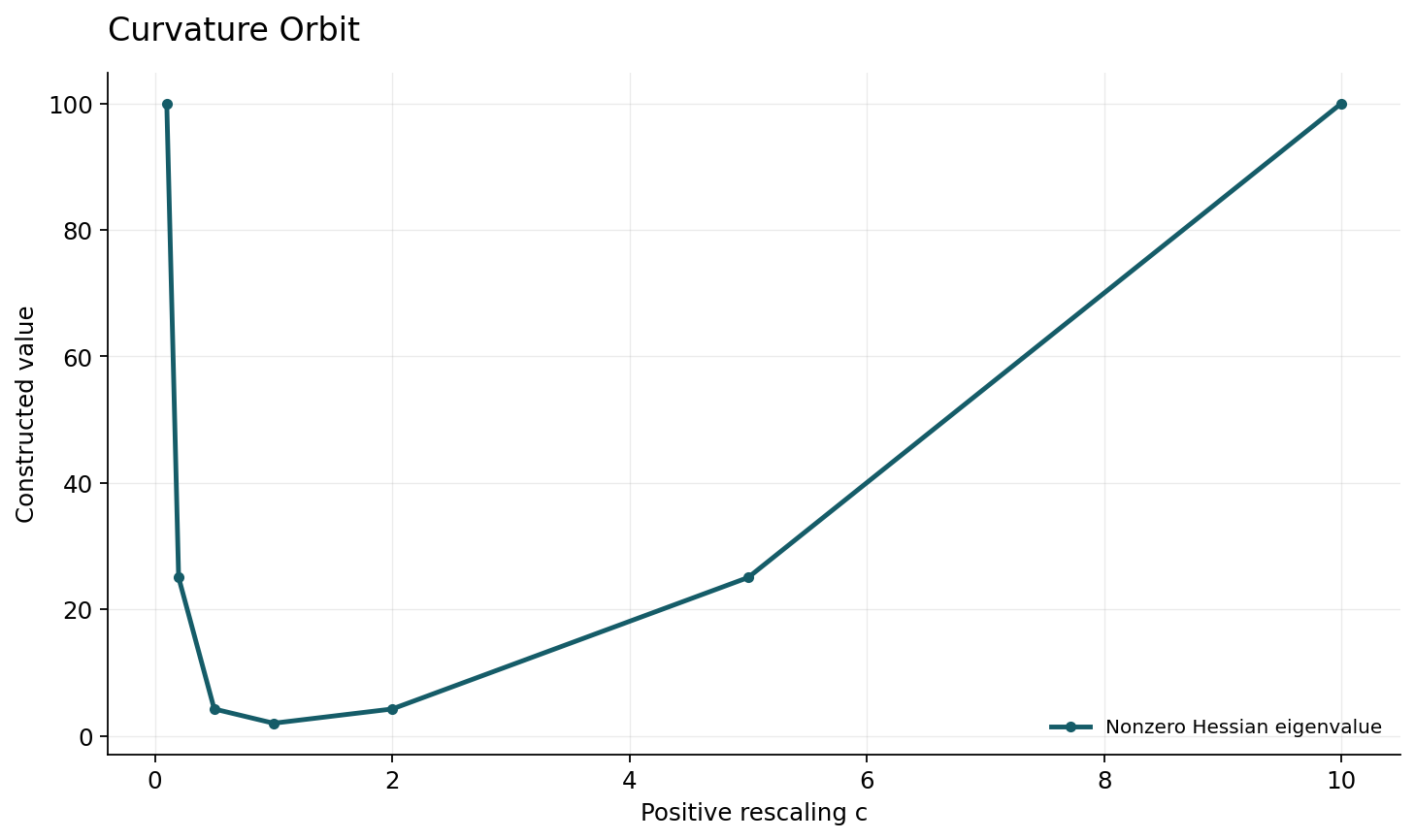
Substituting a=c and b=1/c gives nonzero curvature c squared plus c to the power minus two. Its minimum is two at c=1, and it grows without bound as c tends to infinity or zero. The zero eigenvalue describes the tangent to the symmetry orbit at first order. Its presence does not mean every finite move in that straight tangent direction has zero loss; the exact symmetry path is curved in ordinary parameter coordinates. This detail prevents another common misuse of local geometry. The result is algebraic and exact. A numerical Hessian implementation should reproduce it, but its correctness here does not depend on automatic differentiation, a finite-difference step, or the precision of a plotted contour.
5. What the counterexample refutes and leaves open
The predictor, training loss, test predictions, and statistical risk stay fixed while the largest Hessian eigenvalue changes. Therefore that eigenvalue, without a parameterization convention, cannot be a sufficient statistic for generalization. The conclusion does not depend on choosing an especially favorable test set. It holds because the functions agree pointwise. The example also shows why comparing models after arbitrary layer rescaling can create a spurious geometry ranking.
Several stronger questions remain legitimate. A fixed architecture and training convention may constrain the relevant rescalings in practice. A normalized metric may remove some symmetries. A perturbation distribution motivated by quantization or deployment noise may make parameter sensitivity operationally meaningful even when it is not a universal risk explanation. A bound can combine curvature with scale, margins, or a prior and have a different logical status from raw curvature alone. Those possibilities require their own definitions and evidence. The correct response to a symmetry counterexample is to revise the measurement contract and test the revised claim. Quietly retaining the original scalar while changing its interpretation would make independent replication unnecessarily difficult.
6. Perturbation sets transform with the coordinates
Write the balanced coordinates as (u,v), and transform them to (a,b)=(cu,v/c). A perturbation (delta u, delta v) then corresponds to (c delta u, delta v/c). A Euclidean ball in the balanced coordinates becomes an ellipse in the rescaled coordinates. Corresponding points implement identical perturbed products, because (cu+c delta u)(v/c+delta v/c) equals (u+delta u)(v+delta v).
This identity preserves the loss point by point, including nonlinear cross terms. Consequently the supremum over the transformed ellipse equals the supremum over the original ball whenever the same radius and loss are used. In contrast, applying the same ordinary Euclidean ball independently in every coordinate system changes the set of perturbed functions. A different measured sensitivity is then expected. It describes a different experiment, rather than a contradiction. The practical question is which perturbations are scientifically justified. Additive device noise in physical weights, relative numerical error, and function-space output perturbations need not induce the same geometry. A study should explain why its chosen set represents a relevant uncertainty or intervention before interpreting the result as robustness.
7. Sharpness-aware optimization is an intervention
Foret and colleagues formulate sharpness-aware minimization around neighborhoods of parameters and report empirical gains across selected tasks. This is an algorithmic contribution: the training procedure changes which parameter values are selected. Its effectiveness is evaluated through outcomes of the resulting predictors, not established merely by naming the objective sharpness-aware. The current construction neither reproduces nor overturns those reported benchmark outcomes.
For the toy loss, a neighborhood objective can be defined as the maximum loss within a radius rho around a chosen point. The objective depends on the norm used to define that neighborhood. Transforming coordinates while retaining an unchanged Euclidean radius generally changes the optimization problem. Transforming the perturbation set consistently preserves the underlying problem. This distinction separates an invariance question from an efficacy question. An optimizer may be useful under a deliberately chosen parameter metric, even though its objective is not invariant under every equivalent representation. To investigate why it helps, one should compare training budgets, perturbation radii, achieved fit, and test behavior while holding the interpretation of the intervention stable.
Sources: [3]
8. A figure can conceal the intervention it visualizes
Li and colleagues use filter normalization in loss-landscape visualization, making direction scaling an explicit part of the method. Such choices matter because a two-dimensional slice is not the full loss landscape. Two plotted directions may intersect very different subsets of function space, even when axes carry the same numerical ticks. A wide-looking basin can result from a smaller effective perturbation rather than an intrinsically different predictor.
In the construction, drawing contours over a fixed square around (c,1/c) produces visibly different shapes as c changes. Drawing the corresponding transformed square instead preserves every sampled loss value. Both pictures can be correct. Their captions must explain which comparison they represent. A responsible visualization records the center, directions, normalization, radius, loss reduction, and sampling resolution. If batch-normalization statistics or stochastic layers are involved, it also records their evaluation state. Without those details, another researcher cannot tell whether the figure reflects a property of the trained function, a parameterization convention, or an accidental change in evaluation procedure.
Sources: [4]
9. Scale-aware explanations require complete quantities
Neyshabur and colleagues examine norm, sharpness, robustness, and scale normalization in generalization analysis. Their framing motivates keeping all terms of a proposed explanation visible. Rescaling may reduce one part of an expression while increasing another. Reporting only the favorable factor can turn a meaningful combined quantity into a misleading ranking. In particular, parameter noise and the complexity cost assigned to that noise cannot be independently optimized without changing the meaning of a certificate.
A comparable issue arises in margin-based reasoning. Multiplying all output scores can change a raw margin without changing predicted labels, while a normalized margin accounts for an appropriate scale. The relevant normalization must be specified rather than selected after seeing which version best correlates with test outcomes. This article does not assert that one normalization solves every architecture. It proposes a falsification test: apply transformations known to preserve the evaluated predictor, recompute the proposed measure, and determine which changes are permitted by the theory. If the measure is intentionally coordinate dependent, the paper should say what operational property that dependence represents.
Sources: [5]
10. Correlation across trained models is a separate hypothesis
Jiang and colleagues compare numerous generalization measures under controlled training variations. This kind of broad evaluation addresses a question that a single illustrative contour cannot answer: whether a candidate statistic remains informative when other aspects of training vary. The result of such a study is still conditional on its experimental family. It does not transform an empirical correlation into an unrestricted causal law.
An audit should distinguish within-family prediction from transfer across families. A measure can rank checkpoints of one run while failing across architectures, or correlate with test loss only because both respond to training duration. Stratifying by the intervention helps expose those alternatives. For example, compare geometry after function-preserving rescaling as a negative control, and compare genuinely different training outcomes as the substantive test. The first checks the measurement's interpretation; the second checks its empirical usefulness. Holding a final evaluation set apart from measure selection is essential. Otherwise repeated attempts to discover the best geometry statistic make the reported association another form of adaptive model selection.
Sources: [6]
11. A reproducible finite-radius calculation
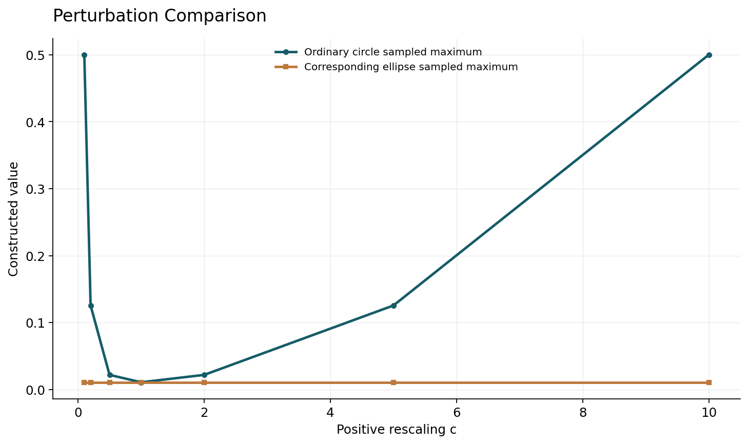
The first scientific figure plots the exact nonzero Hessian eigenvalue for c in a declared positive range. A second calculation samples a circle of radius rho around each representative. For each angle it evaluates the exact nonlinear loss, retaining the largest sampled value. This sampled maximum is a lower bound on the continuous maximum, not a certified maximizer. Increasing angular resolution checks numerical stability of the plotted approximation but does not change that logical status.
The same angle list is then transformed into the corresponding ellipse. Every transformed loss must agree with the balanced-coordinate loss to floating-point tolerance. This is a stronger implementation check than comparing only the largest values, because a maximum can agree accidentally. The receipt includes the largest pointwise discrepancy and the common grid definition. A negative control applies an untransformed circle after rescaling and should show a different result. All values are constructed mathematical examples. They are not sharpness measurements from an empirical neural-network benchmark, and the figure does not attach invented test errors to any of the curves.
12. A study design that can support a stronger claim
Choose the application loss, data sampling unit, architecture, normalization state, and final evaluation distribution before comparing geometry. Define the perturbation metric and radius with a scientific rationale. Report the exact algorithm used to estimate a supremum or Hessian quantity, including stopping conditions and numerical tolerances. If the estimator finds a large loss increase, that witnesses vulnerability within its searched set. Failure to find one does not certify that no larger increase exists.
Run function-preserving transformations where available, checking predictions before and after each transformation. Then run matched training interventions, recording achieved training loss, compute, learning-rate schedule, regularization, and validation selection. A difference in generalization should be attributed to the full procedure unless a further causal design isolates geometry. Include calibration or subgroup metrics only when they answer a declared application question; a lower aggregate test error does not establish every form of reliability. Finally, publish unsuccessful transformations and optimizer failures. Excluding the cases where the proposed explanation breaks can make a measure appear stable precisely by hiding its most informative counterexamples.
A practical symmetry test also needs a tolerance on functional equivalence. Compare logits or real-valued outputs over a declared probe set, not merely hard labels: two networks can agree on classifications while having different margins and losses. For an exact algebraic symmetry the function-level equality follows analytically, as in the construction. For a complex implementation, discrepancies can arise from finite precision, normalization state, or a transformation that was only approximately a symmetry. Report those discrepancies before interpreting any change in geometry. If the transformed model has different outputs, it no longer provides a clean same-predictor negative control. This ordering of checks prevents an attractive but invalid invariance demonstration from becoming evidence about a property it did not actually hold fixed.
13. Numerical and conceptual limitations
The two-parameter product has no learned high-dimensional representation, no stochastic gradient noise, and no finite-sample estimation problem. It establishes a logical limitation on an unnormalized geometry claim. It cannot predict the magnitude of a large-batch generalization gap, select a useful radius for a vision model, or decide between practical sharpness-aware variants. Those questions require additional analysis or experiments with explicitly controlled procedures.
The finite-radius figure is also limited by its angular grid. Its job is to show transformed-set equality and an ordinary-ball contrast, not certify a difficult high-dimensional adversarial maximum. The Hessian calculation holds at exact interpolation. Away from that manifold, residual-dependent second derivatives enter the Hessian and change its eigenvalues. The function-preserving transformation still preserves predictions, but a curvature formula must be rederived at the actual point. Nonhomogeneous activations, weight decay, normalization layers, and architectural constraints can alter which rescalings are symmetries of a complete training objective. A useful audit checks these conditions directly instead of assuming that a scalar toy transformation applies unchanged to every network.
14. Geometry earns meaning through a measurement contract
Loss geometry can help diagnose optimization and motivate training algorithms. Its scientific value increases when the measurement contract identifies coordinates, perturbations, evaluated loss, and the relationship to the predictor. The exact construction offers a compact checklist: identical functions, changing ordinary Hessian curvature, invariant corresponding perturbations, and a clear distinction between coordinate dependence and algorithmic effectiveness. Each statement is separately testable.
Future work can ask which symmetry-aware metrics remain computationally practical, which perturbation models match deployment errors, and which geometry diagnostics predict useful outcomes outside the family in which they were chosen. A successful answer should survive negative controls and preserve uncertainty about untested regimes. Calling one basin flatter is only the beginning of that argument. The stronger conclusion requires showing what variation has been measured, why it matters for the task, and what evidence connects it to new observations. That standard allows both constructive algorithm design and skeptical examination of proposed explanations without confusing a convenient visualization with a universal account of deep learning.
Core equations and definitions
(1) Declared scalar construction; every ab=1 gives the same function.
(2) At zero residual the Hessian is an outer product.
(3) Euclidean curvature varies without changing any prediction.
(4) The same perturbation experiment maps a ball to an ellipse.
(5) Exact invariance including finite nonlinear cross terms, not only a local Taylor approximation.
Constructed analytical figures
Comparison and reporting contract
| Quantity | Preserved along ab=1? | Interpretation |
|---|---|---|
| All predictions | Yes | Same function for every input |
| Population prediction risk | Yes, when defined | Any fixed distribution and prediction loss |
| Largest Euclidean Hessian eigenvalue | No | Depends on chosen coordinates |
| Corresponding transformed perturbation loss | Yes | Same set of perturbed functions |
| Untransformed Euclidean-ball loss | Generally no | Different perturbation intervention |
Evaluation protocol
- Check algebraic Hessian eigenvalues over positive c.
- Evaluate exact losses on a fixed angular grid and compare every transformed perturbation.
- Use untransformed circles as a negative control; label maxima as grid lower bounds.
- For real models, preregister metric and matched training/evaluation procedures.
Limitations
- Two-parameter construction is not an empirical deep-network experiment.
- Finite angular sampling does not certify the continuous supremum.
- Source abstracts support only attributed high-level scope; no source benchmark or theorem proof is independently replicated.
Open research questions
- Which symmetry-aware metrics remain useful under realistic normalization and finite precision?
- Which parameter perturbation distributions model actual deployment noise?
- Do chosen geometry diagnostics transfer beyond the training families used to select them?
Evidence and its boundaries
- Equivalent rectifier-network parameterizations can have different sharpness; a parameter-space measure needs a specified representation.
- [1] — Only the inspected source scope is used; no source benchmark or proof is claimed as independently reproduced. Inspected: Primary arXiv title, authors, version history and abstract inspected on 2026-10-27.
- Reports experiments relating batch size and a selected sharpness measure; this is empirical evidence within its tested setup, not an invariant law.
- [2] — Only the inspected source scope is used; no source benchmark or proof is claimed as independently reproduced. Inspected: Primary arXiv title, authors, version history and abstract inspected on 2026-10-27.
- Introduces a neighborhood min-max training objective and reports benchmark results; the current article does not reproduce those benchmarks.
- [3] — Only the inspected source scope is used; no source benchmark or proof is claimed as independently reproduced. Inspected: Primary arXiv title, authors, version history and abstract inspected on 2026-10-27.
- Uses filter normalization for loss-landscape comparisons, showing that a visualization's direction scale is an explicit methodological choice.
- [4] — Only the inspected source scope is used; no source benchmark or proof is claimed as independently reproduced. Inspected: Primary arXiv title, authors, version history and abstract inspected on 2026-10-27.
- Studies norm, sharpness, robustness, scale normalization, and their relation to generalization; no single unnormalized Hessian scalar is licensed as a universal certificate.
- [5] — Only the inspected source scope is used; no source benchmark or proof is claimed as independently reproduced. Inspected: Primary arXiv title, authors, version history and abstract inspected on 2026-10-27.
- Evaluates many proposed complexity measures under controlled training variations; supports careful experimental comparison rather than universal extrapolation.
- [6] — Only the inspected source scope is used; no source benchmark or proof is claimed as independently reproduced. Inspected: Primary arXiv title, authors, version history and abstract inspected on 2026-10-27.
References
- Sharp Minima Can Generalize For Deep Nets
Laurent Dinh, Razvan Pascanu, Samy Bengio, Yoshua Bengio. Primary arXiv paper record (2017). https://arxiv.org/abs/1703.04933Source scope
Primary arXiv title, authors, version history and abstract inspected on 2026-10-27.
- On Large-Batch Training for Deep Learning: Generalization Gap and Sharp Minima
Nitish Shirish Keskar, Dheevatsa Mudigere, Jorge Nocedal, Mikhail Smelyanskiy, Ping Tak Peter Tang. Primary arXiv paper record (2017). https://arxiv.org/abs/1609.04836Source scope
Primary arXiv title, authors, version history and abstract inspected on 2026-10-27.
- Sharpness-Aware Minimization for Efficiently Improving Generalization
Pierre Foret, Ariel Kleiner, Hossein Mobahi, Behnam Neyshabur. Primary arXiv paper record (2021). https://arxiv.org/abs/2010.01412Source scope
Primary arXiv title, authors, version history and abstract inspected on 2026-10-27.
- Visualizing the Loss Landscape of Neural Nets
Hao Li, Zheng Xu, Gavin Taylor, Christoph Studer, Tom Goldstein. Primary arXiv paper record (2018). https://arxiv.org/abs/1712.09913Source scope
Primary arXiv title, authors, version history and abstract inspected on 2026-10-27.
- Exploring Generalization in Deep Learning
Behnam Neyshabur, Srinadh Bhojanapalli, David McAllester, Nathan Srebro. Primary arXiv paper record (2017). https://arxiv.org/abs/1706.08947Source scope
Primary arXiv title, authors, version history and abstract inspected on 2026-10-27.
- Fantastic Generalization Measures and Where to Find Them
Yiding Jiang, Behnam Neyshabur, Hossein Mobahi, Dilip Krishnan, Samy Bengio. Primary arXiv paper record (2019). https://arxiv.org/abs/1912.02178Source scope
Primary arXiv title, authors, version history and abstract inspected on 2026-10-27.