
When Computation Should Run: Carbon-Aware Scheduling under Deadlines and Forecast Error
Scheduling flexibility can lower attributed emissions, but only a defined baseline, feasible deadline and credible carbon signal make the result interpretable.
English original. Translations of this new review are not yet available.
Abstract
Carbon-aware scheduling uses flexibility in when and where computation runs to change its energy-related emissions. The apparent simplicity of choosing low-carbon hours hides several distinct problems: identifying an appropriate carbon signal, preserving deadlines, predicting future load, accounting for migration and idle resources, and separating operational from embodied impacts. This review synthesizes six primary research and standards sources while developing a fully specified finite scheduling example. Three identical one-kilowatt-hour jobs are assigned to six capacity-limited slots. Exhaustive enumeration gives realized emissions of 1,350 grams for immediate execution, 990 grams for a forecast-selected schedule and 600 grams for the hindsight optimum. The example illustrates both the value of flexibility and the danger of presenting perfect-information savings as online performance. A bounded-error calculation shows how forecast error limits a regret statement, while deadline relaxation exposes the feasible-set mechanism behind lower offline cost. We then distinguish attributional accounting from causal grid effects and explain why delaying work can increase energy consumption or require additional infrastructure. The proposed evaluation uses time-separated forecasts, explicit completion constraints and lifecycle sensitivity analysis. The resulting claim is conditional: carbon-aware placement is useful when its flexibility, accounting boundary and forecast quality are demonstrated together, rather than inferred from an attractive intensity curve.
In this paper
- 1. A scheduling decision needs a carbon objective
- 2. Flexibility is an application property
- 3. Renewable matching and grid-carbon accounting
- 4. A six-slot example that can be enumerated
- 5. Three schedules answer three different questions
- 6. A forecast-error bound and its weakness
- 7. Deadlines define the feasible set
- 8. Risk-aware planning is still assumption-dependent
- 9. Energy efficiency and carbon timing can conflict
- 10. Operational savings and embodied infrastructure
- 11. A functional unit prevents disappearing work
- 12. Spatial movement adds constraints
- 13. An experiment that respects time
- 14. What the finite model contributes
1. A scheduling decision needs a carbon objective
A scheduler cannot optimize carbon in the abstract. It needs a quantity associated with a unit of execution at a particular time and place. That quantity may describe an attributed share of grid emissions, a modeled marginal effect of additional demand or the availability of a dedicated renewable supply. These are different objectives. Selecting the smallest number from one series does not establish that every other interpretation of emissions has improved.
The initial specification should identify the system boundary, functional unit and baseline. Is the task to finish a fixed batch of jobs, serve a fixed number of requests or deliver a continuously available service? Are facility overheads, network transfers and idle machines included? Is the alternative immediate execution on the same hardware or another feasible schedule? Without these choices, an emissions reduction can be produced by changing what is counted. The analysis below fixes a narrow operational accounting model first, then examines what that model leaves unresolved.
2. Flexibility is an application property
The work on Carbon-Aware Computing for Datacenters describes Google's use of forecasts and virtual capacity curves to shape temporally flexible workloads while preserving daily capacity. It provides evidence that a large operational system can act on such signals. The relevant scope is flexible work under that management framework; it does not establish that arbitrary interactive requests can be delayed without consequence.
For a new workload, flexibility must be discovered or specified at the job level. A deadline is not the only restriction: release times, dependencies, checkpoint boundaries and data availability can constrain execution. A batch that is nominally due at midnight may still require an early stage to produce data for a downstream service. Treating its entire compute budget as freely movable would create a fictitious optimization opportunity. A scheduling study should therefore publish the admissible placements or the rule that constructs them, not only the final carbon-weighted utilization trace.
Sources [1]
3. Renewable matching and grid-carbon accounting
GreenSlot schedules batch work around predicted solar availability and deadlines; GreenHadoop applies renewable-aware scheduling in a data-processing framework. These primary studies motivate the use of temporal flexibility, but their renewable-supply and electricity-cost objectives should not be silently equated with every modern grid-carbon objective. A reduction in purchased electricity cost is not necessarily the same percentage reduction in emissions.
The distinction becomes concrete when a grid has cheap but carbon-intensive generation, or when a site owns renewable output that would otherwise be exported. Moving computation to a sunny hour can change both local consumption and the power delivered elsewhere. An attributional study can report the emissions assigned under its chosen convention. A causal claim about avoided grid emissions requires a model of the counterfactual electricity system. The two can be useful together, but their denominators and assumptions should remain visible. This article's finite example uses a declared intensity series and makes no grid-dispatch claim.
4. A six-slot example that can be enumerated
Consider six one-hour slots, indexed zero through five. Three independent jobs are available at the beginning, each requires one slot, and each consumes exactly one kilowatt-hour. At most one job can execute in a slot, and all three must complete by the end of slot five. There are twenty feasible choices of three occupied slots. Jobs are interchangeable in this example, so permutations of job identities do not create additional cost-distinct schedules.
The forecast intensities are 500, 400, 100, 80, 300 and 600 grams of carbon-dioxide equivalent per kilowatt-hour. The realized intensities are 500, 400, 450, 420, 120 and 80 in the same units. These are synthetic sequences selected to expose forecast error, not observations from an electricity market. The model excludes idle energy, migration, restart costs, embodied emissions and demand-dependent changes in grid intensity. Its limited scope makes every comparison exact and its exclusions straightforward to inspect.
5. Three schedules answer three different questions
Immediate execution occupies slots zero, one and two, producing 1,350 grams under the realized signal. Optimizing the forecast selects slots two, three and four, whose forecast sum is 480 grams but whose realized sum is 990 grams. Optimizing with perfect knowledge of the realized signal selects slots one, four and five, producing 600 grams. The supplied program checks all twenty feasible subsets, rather than assuming that visually adjacent low values form the optimum.
The forecast policy improves on immediate execution in this example, yet remains 390 grams above the hindsight optimum. These statements answer different questions. The first compares two feasible decisions under one realized sequence. The second measures the cost of imperfect information relative to an oracle. Neither is a general performance guarantee for an online scheduler. In particular, presenting the 600-gram result as achievable forecast-based performance would replace uncertainty with knowledge that the decision maker did not possess.
6. A forecast-error bound and its weakness
Suppose every slot's forecast error is bounded in absolute value by epsilon and every feasible schedule uses exactly E kilowatt-hours. If the selected schedule minimizes forecast cost over the same feasible set as the true optimum, its realized regret is at most twice E times epsilon. The argument compares each schedule's forecast and realized costs, then uses forecast optimality. It does not require the particular six-slot values, but it does require the declared common feasible set and energy accounting.
Here E is three and the largest signal error is 520 grams per kilowatt-hour. The resulting bound is 3,120 grams, much looser than the actual 390-gram regret. A valid bound can therefore be practically uninformative. A useful improvement might exploit where errors occur, their dependence across hours or the margin between competing schedules. Such refinements need assumptions that can be tested on held-out forecasts. A smaller reported bound obtained by ignoring unfavorable forecast errors would not be an improvement in reliability.
7. Deadlines define the feasible set
With only the first three slots available, all jobs must run immediately and the realized optimum is 1,350 grams. Allowing four slots lowers the offline optimum to 1,270 grams; allowing five lowers it to 940 grams; allowing all six lowers it to 600 grams. This monotonicity follows from nesting: every schedule feasible under a shorter horizon remains feasible under a longer one. The result is a property of the offline model, not evidence that delaying an actual application always helps.
A deadline constraint should be checked for every job, not only on aggregate compute delivered. Preserving a day's total capacity can coexist with a particular job missing its deadline if release times or dependencies are ignored. For heterogeneous work, a scheduler must account for job-specific duration, resource needs and placement restrictions. A simulation that quietly drops jobs when capacity is insufficient can achieve attractive carbon results by failing to perform the required work. Completion rate and deadline violations therefore belong beside every emissions number.
8. Risk-aware planning is still assumption-dependent
Hall and colleagues formulate carbon-aware load shaping with probabilistic performance guarantees and distributionally robust optimization, separating planning from real-time placement. The inspected primary abstract describes simulation-based validation and the use of historical load information. That evidence supports a specific risk-aware research direction; it should not be relabeled as a proof that all forecast-driven production workloads meet their service levels.
A guarantee is meaningful only with its uncertainty model, feasibility conditions and probability interpretation intact. A statement about performance under a distributional ambiguity set may fail when the real process lies outside that set. Rare deadline failures also require enough independent or appropriately modeled observations to estimate. For an operational evaluation, record the forecast available at decision time and the prediction interval or uncertainty set actually used. Reconstructing a forecast later from revised data creates look-ahead leakage and can make a fragile scheduler appear consistently well informed.
Sources [3]
9. Energy efficiency and carbon timing can conflict
Delaying work can change total energy use. A machine may remain powered while waiting, a checkpoint may write substantial data, or a job may lose locality after migration. Conversely, batching delayed work can permit some resources to sleep. These effects mean that a fixed-energy scheduling model is a starting point, not a universal description. The comparison should measure or model the additional energy caused by the policy, rather than multiplying the original energy by a more favorable intensity.
For a simple threshold argument, let a move save delta-c grams per kilowatt-hour on E kilowatt-hours of useful work but incur extra emissions M from migration and waiting. The move improves the chosen accounting objective only when E times delta-c exceeds M. This does not require a sophisticated optimizer, but it prevents a common accounting error: charging the original schedule for all energy while treating the optimized schedule's coordination as free. If M is uncertain, the decision margin should reflect that uncertainty.
10. Operational savings and embodied infrastructure
Carbon Explorer analyzes combinations of renewable capacity, storage and workload scheduling while including operational and embodied effects. It motivates treating infrastructure choices as part of the system rather than assuming that extra hardware is carbon-free. The inspected preprint record also differs in title and author ordering from the final conference record; this article cites the inspected preprint explicitly rather than blending metadata across versions.
A scheduler may require extra capacity to concentrate work into favorable hours. If that capacity would not otherwise exist, its manufacturing impact can matter to the comparison. Attribution across a hardware lifetime is not identical to a causal claim that one scheduling decision caused a purchase. Both questions can be analyzed, but the allocation rule and counterfactual should be stated. Sensitivity to utilization and service life is especially important: a low operational intensity does not automatically offset a large amount of rarely used equipment.
Sources [2]
11. A functional unit prevents disappearing work
The Software Carbon Intensity specification defines a rate using operational and embodied emissions divided by a functional unit and requires an explicit boundary. Its accounting framework is useful for making comparisons auditable. A lower score should be interpreted together with the specified service quantity and quality, rather than as an abstract environmental label. This article uses the inspected version 1.1.0 as a methodological source.
For computing, an acceptable functional unit might be one completed query at a stated latency and accuracy, or one finished analysis on a fixed dataset. Defining the unit as one attempted request can reward a system that quickly rejects difficult work. Defining it as one arithmetic operation can reward redundant computation or conceal an algorithmic improvement. The functional unit should remain stable while the implementation changes. Reporting total emissions as well as the rate also helps detect rebound: a lower per-unit value can coexist with a larger total footprint if workload volume increases sufficiently.
Sources [5]
12. Spatial movement adds constraints
Moving work between regions introduces data-transfer time, network energy, data-location restrictions and possibly a different hardware efficiency curve. A low-intensity destination is not necessarily the lowest-emissions destination after these terms are included. The placement problem should therefore separate location feasibility from cost. An infeasible destination should not appear as an attractive option that is rejected only in a footnote.
The workload's state can dominate the decision. A stateless job with a small input may move cheaply, while a computation attached to a large dataset may require substantial transfer or duplicate storage. A migration policy also needs a recovery rule if a transfer fails halfway. The proposed evaluation records transferred bytes, duplicated work and the time at which the destination becomes ready, then checks deadlines against that actual timeline. A scheduler should receive credit only for completed work under the same service contract as the baseline, including failed moves and retries.
13. An experiment that respects time
A credible retrospective study divides data chronologically. The scheduler uses only forecasts and workload information available before each decision, while the evaluator later uses realized outcomes. Training and tuning periods should precede the held-out period. Revisions to grid data, missing intervals and timezone conversions should be recorded. A result based on an idealized signal can still be useful as an upper opportunity estimate, provided that it is labeled accordingly.
The baseline should be a feasible policy that performs the same work, such as immediate execution or an existing deadline-aware scheduler. Report emissions, energy, completion, deadline violations and peak capacity together. Repeat the comparison across seasons, load levels and forecast-error regimes, including periods with little useful flexibility. Statistical uncertainty should respect temporal dependence rather than treating every hour as an independent experiment. The central question is whether the policy delivers a repeatable service-preserving improvement under realistic information, not whether one selected week contains low-carbon hours.
14. What the finite model contributes
The supplied program demonstrates a small number of exact propositions. It enumerates all twenty schedules, verifies the forecast-selected and hindsight costs, checks the bounded-error inequality and confirms that relaxing the deadline cannot worsen the offline optimum. A separate finite permutation check compares exhaustive optimization with the sorted-cost solution for equal-energy jobs. These checks establish the arithmetic of this model, not the environmental impact of a real deployment.
The model's value is diagnostic. If an implementation reports savings larger than its perfect-information opportunity under the same boundary, something about the boundary, baseline or workload accounting has changed. If it reports no savings despite substantial modeled opportunity, forecast error, capacity constraints or overhead may explain the gap. The next research step is to quantify those residuals with time-correct data. A strong carbon-aware scheduling claim therefore includes both the opportunity that flexibility creates and the costs, uncertainty and service restrictions that prevent all of that opportunity from being realized.
A further check is to audit units at every interface. Power sampled in watts must be integrated over time before it becomes energy, and an intensity in grams per kilowatt-hour must not be multiplied directly by a watt reading. Missing intervals need a declared treatment. These apparently mundane choices can dominate a small reported saving. The evaluation package should therefore retain the unit conversions and interval boundaries alongside the optimizer output, allowing a reviewer to reproduce the accounting without relying on an opaque dashboard.
Mathematical model
(1) Attributed operating emissions in grams, with schedule energy e_t in kWh and intensity c_t in gCO2e/kWh. This formula alone does not identify marginal grid effects.
(2) Forecast-optimal schedule over a fixed feasible set F containing the same required work and deadline constraints as the realized comparison.
(3) If every feasible schedule uses total energy E and max_t|c_t-c_hat_t|<=epsilon, compare forecast and actual costs twice and use forecast optimality.
(4) Deadline relaxation cannot worsen an offline optimum when all other assumptions and costs are unchanged.
(5) A move is beneficial under the stated accounting only when avoided operating emissions exceed additional migration, waiting and other included emissions M.
Reproducible analytical figures
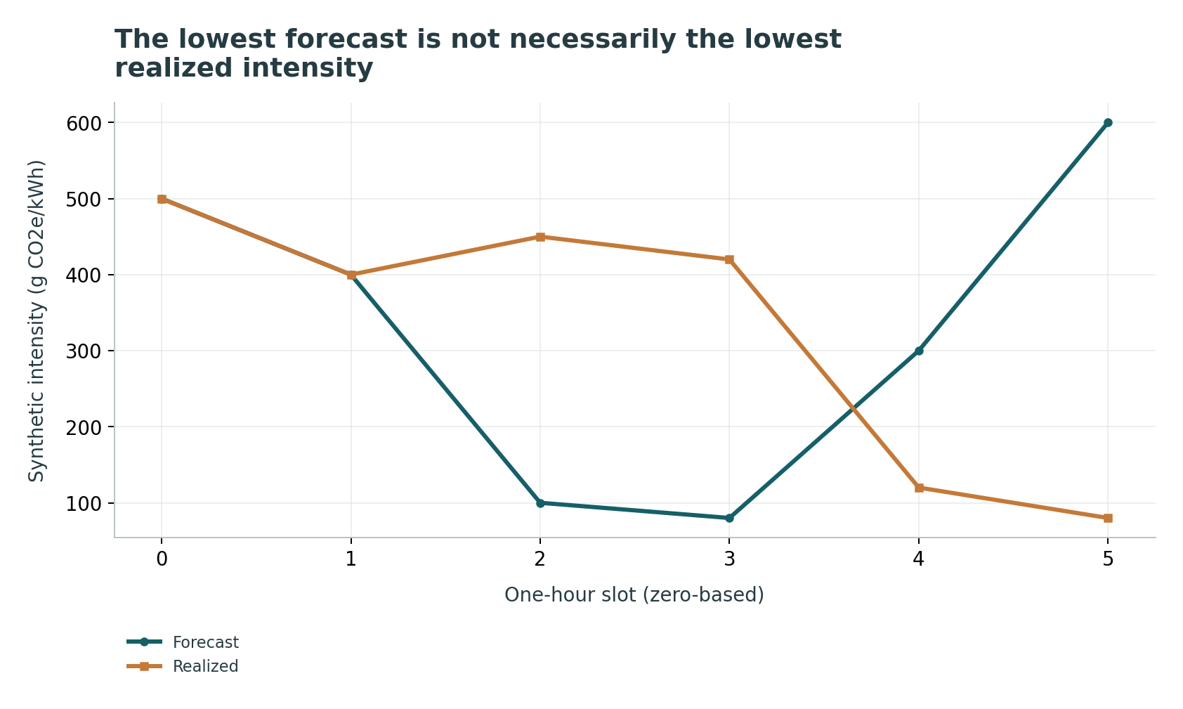
Assumptions: No idle, migration, start-up or embodied emissions in this narrow example; All jobs identical and independent

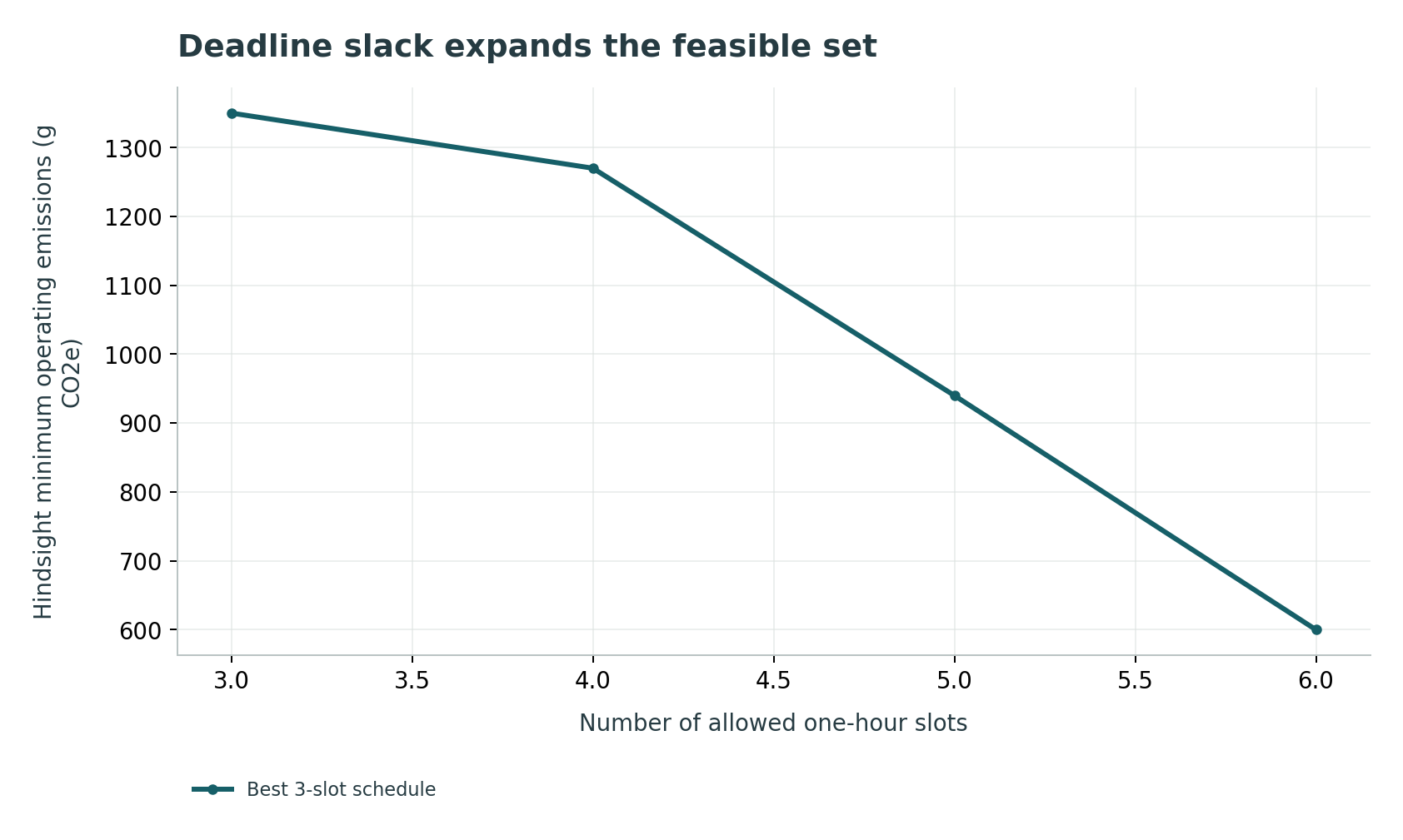
Assumptions: Three unit jobs; capacity one each slot; One kWh per job; no switching overhead

Executed finite checks
3 check groups passed. The listed cases validate this model; they are not independent experiments or system benchmarks.
- Forecast policy and hindsight optimum by exhaustive enumeration · 20 cases. All feasible 3-of-6 schedules; actual emissions 990 g versus oracle 600 g and immediate execution 1,350 g.
- Equal-energy sorting optimum cross-checked against enumeration · 120 cases. Every permutation of five distinct costs, selecting two slots.
- Deadline relaxation and bounded-error regret · 4 cases. Larger feasible sets cannot worsen the offline optimum; regret 390 g <= 6 * 520 g.
Comparison
| Quantity | Necessary interpretation | Common confusion |
|---|---|---|
| Forecast-selected emissions | Realized cost of a decision made with forecast data | Using the forecast cost as the observed result |
| Oracle optimum | Perfect-information opportunity under fixed constraints | Calling hindsight achievable online performance |
| Average intensity | Attribution according to the chosen convention | Equating it with a causal marginal effect |
| SCI rate | Emissions per declared functional unit | Hiding service reduction or total growth |
| Deadline compliance | Every required job meets its contract | Reporting only total daily capacity |
Proposed validation protocol
- Fix required work, deadlines, release times and allowed locations.
- Declare operational and embodied boundaries and functional unit.
- Archive forecasts exactly as available at each decision time.
- Separate training, tuning and evaluation chronologically.
- Check that every baseline and candidate completes the same work.
- Enumerate or optimize a hindsight bound under identical constraints.
- Include idle, migration, restart and storage energy when applicable.
- Test forecast misses, capacity shortage and failed migrations.
- Report energy, emissions, completion, latency and peak capacity together.
- Publish sensitivity to intensity convention, hardware lifetime and temporal dependence.
Limitations
- The six-slot signals are synthetic and do not model any actual electricity system.
- All jobs in the finite example are identical and available at time zero.
- The fixed-energy regret bound can be loose and does not capture changing feasible sets.
- No grid dispatch model or marginal-emissions causal estimate is supplied.
- No production scheduler or infrastructure lifecycle assessment was executed.
- The source set is a focused synthesis, not a complete review of carbon-aware computing.
Open research questions
- Which forecast-error summaries yield useful regret bounds without ignoring temporal dependence?
- How much additional capacity is justified by temporal carbon flexibility after embodied impacts are included?
- Can service-level contracts expose useful flexibility without giving a scheduler permission to drop or silently degrade work?
Evidence and its boundaries
- [1] Google's system uses forecasts and capacity shaping for flexible workloads.
- Not a guarantee for arbitrary interactive requests. Inspected: arXiv:2106.11750v1 abstract and system summary.
- [2] Carbon Explorer considers operational and embodied effects across infrastructure choices.
- Cited preprint metadata is kept separate from final proceedings metadata. Inspected: arXiv:2201.10036v3 record and abstract.
- [3] Risk-aware load shaping separates planning and real-time placement.
- Abstract reports simulation validation; no independent theorem audit is claimed. Inspected: arXiv:2410.21510v3 abstract, scope and version record.
- [4] GreenSlot schedules batch jobs around solar forecasts and deadlines.
- Renewable matching and cost savings are not automatically marginal carbon savings. Inspected: Rutgers DCS-TR-686 record and abstract.
- [5] SCI uses a defined boundary and functional unit including operational/embodied terms.
- A score does not replace total emissions or causal analysis. Inspected: SCI specification 1.1.0 introduction and methodology.
- [6] GreenHadoop uses bounded scheduling flexibility in a data-processing framework.
- Published evaluation is not rerun and not generalized to all grids. Inspected: Author-hosted EuroSys12 PDF abstract and introduction.
References
- Carbon-Aware Computing for Datacenters
Ana Radovanovic, Ross Koningstein, Ian Schneider, Bokan Chen, Alexandre Duarte, Binz Roy, Diyue Xiao, Maya Haridasan, Patrick Hung, Nick Care, Saurav Talukdar, Eric Mullen, Kendal Smith, MariEllen Cottman, Walfredo Cirne. arXiv:2106.11750v1 (2021). https://arxiv.org/abs/2106.11750v1
DOI: 10.48550/arXiv.2106.11750Source access and scope
Primary bibliographic record and abstract inspected; quantitative results are not independently replicated.
- Carbon Explorer: A Holistic Approach for Designing Carbon Aware Datacenters
Bilge Acun, Benjamin Lee, Fiodar Kazhamiaka, Kiwan Maeng, Manoj Chakkaravarthy, Udit Gupta, David Brooks, Carole-Jean Wu. arXiv:2201.10036v3; first submitted 2022 (2023). https://arxiv.org/abs/2201.10036v3Source access and scope
Preprint record/abstract inspected. Title and author order follow this record, not the differently titled final ASPLOS proceedings entry.
- Carbon-Aware Computing for Data Centers with Probabilistic Performance Guarantees
Sophie Hall, Francesco Micheli, Giuseppe Belgioioso, Ana Radovanović, Florian Dörfler. arXiv:2410.21510v3; first submitted 2024 (2025). https://arxiv.org/abs/2410.21510v3
DOI: 10.48550/arXiv.2410.21510Source access and scope
Primary bibliographic record and abstract inspected; quantitative results are not independently replicated.
- GreenSlot: Scheduling Energy Consumption in Green Datacenters
Inigo Goiri, Kien Le, Md E. Haque, Ryan Beauchea, Thu Nguyen, Jordi Guitart, Jordi Torres, Ricardo Bianchini. Rutgers University, DCS-TR-686 (2011). https://scholarship.libraries.rutgers.edu/esploro/outputs/technicalDocumentation/GreenSlot-Scheduling-Energy-Consumption-in-Green/991031550040804646
DOI: 10.7282/T3XK8K29Source access and scope
Primary bibliographic record and abstract inspected; quantitative results are not independently replicated.
- Software Carbon Intensity (SCI) Specification, version 1.1.0
Green Software Foundation. Green Software Foundation (2026). https://sci.greensoftware.foundation/Source access and scope
Official specification version 1.1.0 inspected; year denotes access on 2026-10-25, not original publication.
- GreenHadoop: Leveraging Green Energy in Data-Processing Frameworks
Íñigo Goiri, Kien Le, Thu D. Nguyen, Jordi Guitart, Jordi Torres, Ricardo Bianchini. EuroSys (2012). https://personals.ac.upc.edu/jguitart/HomepageFiles/EuroSys12.pdf
DOI: 10.1145/2168836.2168843Source access and scope
Author-hosted original PDF title, abstract and introductory problem scope inspected.