
Deep Learning Uncertainty / DEEP LEARNING II
When Many Models Share One Mistake: Error Correlation and Epistemic Signals in Deep Ensembles
Exact covariance and mixture constructions explain ensemble gains, saturation and the limits of disagreement under distribution shift.
English original. Translations of this new review are not yet available.
Abstract
An ensemble's member count is not its effective number of independent error sources. This analytical review examines how shared bias, error covariance, predictive mixtures and model-selection diversity affect the interpretation of deep-ensemble uncertainty. An exact equicorrelated error construction yields a variance floor and an effective-size formula, while a shared-error counterexample shows that zero disagreement can coexist with large error. Reproducible finite checks and a shift-evaluation protocol distinguish uncertainty relative to the selected member distribution from a guarantee about all plausible unknown predictors.
In this paper
- 1. The ensemble is only as diverse as its errors
- 2. Practical deep ensembles establish an empirical baseline
- 3. Define the random error before taking its covariance
- 4. A variance floor defines effective ensemble size
- 5. A finite latent construction verifies the formula
- 6. Shared bias is invisible to disagreement
- 7. Predictive mixture variance has two terms
- 8. Classification disagreement is information within a model
- 9. Function diversity matters more than parameter distance
- 10. A Bayesian interpretation needs a declared approximation
- 11. Efficient diversity and hyperparameter search have costs
- 12. Dataset shift tests coverage of alternatives
- 13. Reproducible arithmetic and a full empirical protocol
- 14. Agreement is evidence about the ensemble's scope
1. The ensemble is only as diverse as its errors
A collection of models can disagree substantially in parameter space while making almost the same predictions, or look different on familiar observations while sharing the same failure outside them. Counting members therefore gives an incomplete account of an ensemble's statistical benefit. What matters for averaging error is the joint distribution of their errors, including shared bias and covariance. What matters for an uncertainty signal is which plausible alternatives the ensemble actually represents.
This article focuses on those two questions rather than offering another general survey of probability calibration. Selected primary deep-ensemble papers provide empirical and methodological context. Exact scalar error constructions isolate covariance effects, and finite predictive mixtures expose what disagreement measures. A counterexample then shows why identical wrong members provide no warning about a shared failure. No neural training experiment or new uncertainty benchmark is claimed. The purpose is to define an auditable interpretation: uncertainty relative to a specified distribution over selected models, evaluated on specified inputs. Whether that distribution captures the important unknown alternatives is a further empirical and modeling question. Keeping that question visible prevents a low ensemble variance from being mistaken for proof that a prediction is correct.
2. Practical deep ensembles establish an empirical baseline
Lakshminarayanan, Pritzel and Blundell propose a practical deep-ensemble uncertainty procedure and evaluate it on classification, regression and distribution-shift tasks. Their results make independently trained members a useful baseline for uncertainty research. The method's simplicity does not remove the need to specify training randomness, objectives and aggregation. A different collection of models can have a different joint error structure even when its member count matches.
For a new study, record whether members differ by initialization, data resampling, augmentation, architecture or hyperparameters. State whether their predictive distributions or logits are averaged, since these are different operations. Include total training and inference cost, and preserve the selection rule used to choose members. The original paper's reported outcomes are source results, not measurements recreated in this article. Our finite constructions concern a mathematical reason why averaging can help and a reason it can saturate. They do not determine the accuracy or shift sensitivity of a particular image model. A useful baseline remains a hypothesis-generating instrument whose performance must be assessed under the actual task and resource constraints.
Sources: [1]
3. Define the random error before taking its covariance
Fix an input x and its target value f_star. Treat training randomness as the source of variation across members, and write member m's prediction as f_star plus a shared bias b plus a zero-mean error epsilon_m. Assume each epsilon has variance sigma squared and every different pair has covariance rho times sigma squared. These are explicit equicorrelation assumptions for a scalar regression construction, not a universal model of deep-network errors.
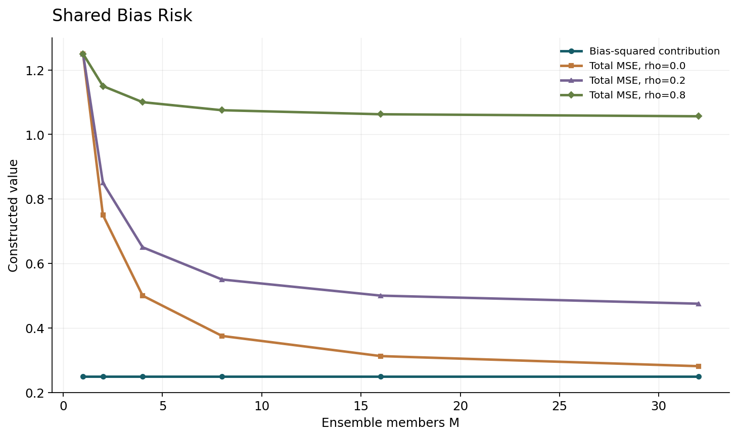
The average member error has mean b. Its variance is the sum of all variances and covariances divided by M squared. There are M diagonal terms and M times M minus one ordered off-diagonal terms, yielding sigma squared times rho plus one minus rho divided by M. Consequently expected squared error equals b squared plus that variance. Averaging reduces the idiosyncratic component but leaves the shared bias and correlated component. This derivation uses neither a held-out empirical correlation estimate nor a Bayesian posterior. It is exact under the declared moments. A real evaluation must specify over what randomness or population its covariance is estimated, because covariance across seeds at one input and covariance of errors across inputs answer different questions.
4. A variance floor defines effective ensemble size
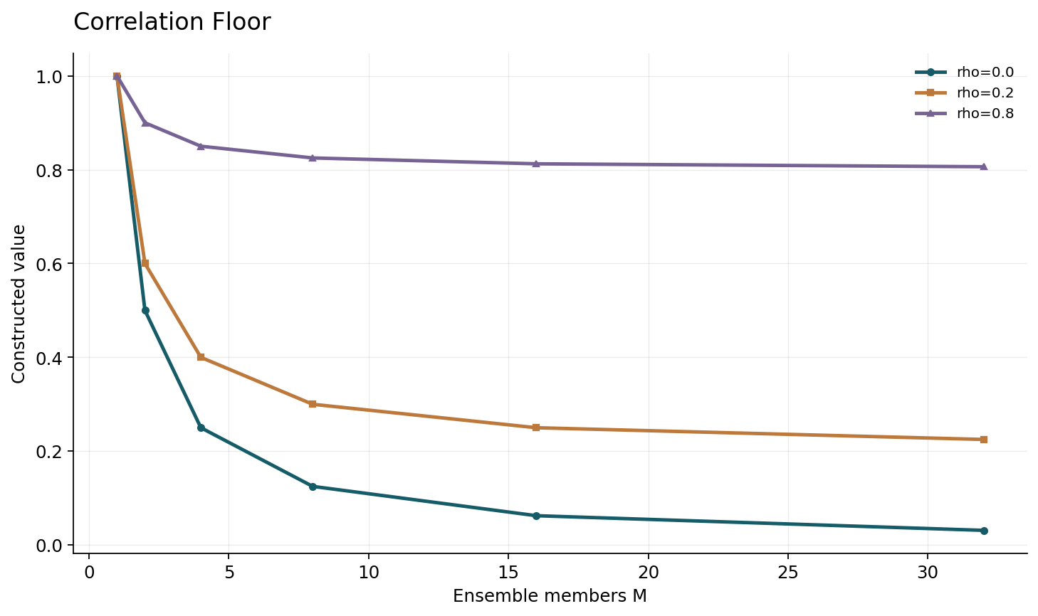
When rho is positive, increasing M cannot reduce variance below rho times sigma squared in this construction. Defining effective size as sigma squared divided by the average's variance gives M divided by one plus M minus one times rho. For rho zero it equals M. For positive rho it approaches one divided by rho as M grows. Thus many highly correlated members can deliver the variance reduction of only a small independent ensemble.
The formula is a diagnostic analogy, not a statement that a real network has a single effective size across all inputs. Correlation can vary by region, subgroup or shift. The same ensemble may provide useful diversity in one region and shared errors in another. Equicorrelation itself has a validity condition: its covariance matrix must be positive semidefinite, requiring rho between minus one divided by M minus one and one for M greater than one. Our figures use only nonnegative rho values, which remain valid over the whole displayed member-count range. Extending a negative rho curve indefinitely without checking this condition would plot an impossible covariance model. Scientific visualization should enforce such domain constraints rather than allowing a mathematically invalid parameter sweep.
5. A finite latent construction verifies the formula
For nonnegative rho, define epsilon_m as square root rho times a shared Rademacher variable Z0 plus square root one minus rho times a member-specific Rademacher variable Zm. All Z variables are mutually independent and equally likely to be minus one or plus one. Each error has mean zero and variance one, while distinct errors have covariance rho. The construction realizes the declared covariance with a finite probability space.
For a modest member count, enumerate every sign vector and calculate the average error directly. Its exact finite expectation and second moment must match the covariance derivation to floating-point tolerance. This is stronger than generating one convenient random sample and observing an approximately matching curve. The enumeration also clarifies what the randomness means: it is a constructed distribution over possible error vectors, not independent labels or training runs from a cited dataset. A negative control duplicates one member's error across all M positions. Its average has unchanged variance, corresponding to perfect correlation. Increasing the displayed number of identical predictions has created no additional error cancellation. This check is simple enough to include in an independent reader's executable verification artifact.
6. Shared bias is invisible to disagreement
Let every member predict two when the true scalar target is zero. Their empirical disagreement variance is zero, but their squared error is four. This exact counterexample shows that agreement cannot certify correctness. It does not claim that deep ensembles are always overconfident or that every out-of-distribution example produces a shared error. It identifies a failure mode that an evaluation must be capable of detecting.
The same issue applies when all members share a representation, training corpus artifact or missing hypothesis. Random seeds explore the procedure's reachable solutions, not necessarily every scientifically plausible predictor. Increasing seeds can improve coverage of that reachable set while leaving a common blind spot untouched. A useful uncertainty study therefore measures prediction error and uncertainty jointly, including regions where members agree and are wrong. It should also inspect whether member selection rewards complementary errors or merely repeated high performance on one development distribution. The finite example separates two achievements: reducing stochastic variability among reasonable predictors and recognizing that the entire model family may be misspecified. The first does not automatically deliver the second.
7. Predictive mixture variance has two terms
Suppose member m supplies a scalar predictive distribution with mean mu_m and variance v_m, and select a member uniformly. The variance of the resulting mixture equals the average v_m plus the average squared deviation of mu_m from their mean. This is the law of total variance for the declared finite mixture. The second term measures disagreement among member means; the first reflects the variances reported within members.
These terms are often associated with aleatoric and epistemic uncertainty, but the labels require interpretation. A reported within-member variance need not equal the true irreducible noise if the member is misspecified or poorly fitted. Between-member disagreement is uncertainty relative to the selected member distribution, not an automatic measure of every unknown function consistent with available evidence. The identity remains mathematically correct even when both interpretations fail. A careful report publishes the predictive likelihood assumptions and evaluates the full mixture as well as its decomposition. It also distinguishes the mixture variance's one-over-M normalization from an unbiased sample-variance estimator using one over M minus one. Those quantities serve different purposes and should not be swapped silently in a plotted uncertainty diagnostic.
8. Classification disagreement is information within a model
For a categorical ensemble, choose member index M uniformly and draw a label from that member's predictive probabilities. The predictive entropy of the averaged distribution minus the average member entropy equals the mutual information between the index and the drawn label in this finite mixture model. It is nonnegative and becomes zero when all member distributions agree. The identity says how much observing the label would reveal about which member generated it.
It does not directly measure information about the unknown correct label mechanism. If every member confidently assigns the same wrong class, both the disagreement information and member entropy can be small. If members disagree because some were deliberately made poor, the information can be large without being useful. This distinction prevents treating diversity as an objective that should be maximized without regard to member quality. The scalar covariance construction and the categorical mixture identity answer different questions; neither supplies a universal decision threshold for out-of-distribution detection. A study should specify the uncertainty score, its intended use, and the alternatives it is expected to distinguish before selecting thresholds on a development set.
9. Function diversity matters more than parameter distance
Fort, Hu and Lakshminarayanan investigate deep ensembles through prediction-space diversity and compare independent initializations with trajectory or subspace samples. Their analysis motivates evaluating functions rather than assuming that widely separated weight vectors make complementary predictions. Neural parameter symmetries and redundant coordinates can produce large parameter distances without equivalent functional differences.
A practical diagnostic measures disagreements and error correlations on declared inputs, including a held-out shift set when relevant. It should retain member quality, because two inaccurate members can be highly diverse for unhelpful reasons. Report pairwise errors, aggregate performance and the incremental contribution of each additional member under a prespecified selection rule. A two-dimensional diversity–accuracy visualization can summarize the explored family but cannot show every unseen failure. The source's empirical hypothesis about modes is not reproduced by our finite covariance example, and the example does not prove how real optimization explores those modes. Keeping these layers separate helps turn a qualitative story about multiple solutions into a measurable claim about which predictions differ and whether averaging those differences improves the intended outcome.
Sources: [3]
10. A Bayesian interpretation needs a declared approximation
Wilson and Izmailov emphasize marginalization and present a probabilistic perspective on deep ensembles and generalization. This provides a useful interpretation of averaging across plausible predictors. An arbitrary set of trained seeds is nevertheless not automatically an exact sample from a specified posterior distribution. To make a stronger Bayesian claim, identify the prior, likelihood, target posterior and approximation procedure, and explain how the selected members relate to it.
The finite mixture remains a well-defined predictive distribution even without that stronger claim. Its uncertainty can be evaluated empirically as the output of a concrete algorithm. Problems arise when a convenient interpretation is presented as an already verified sampling guarantee. For example, uniform member weights may not equal posterior mass weights, and optimizer accessibility need not match posterior probability. These facts do not make the predictor useless; they delimit the inference one can draw from its spread. A transparent paper can report both the practical ensemble procedure and the extent to which its probabilistic interpretation is assumed, approximated or tested. That distinction is especially important when uncertainty is used to decide which predictions should be deferred or investigated.
Sources: [4]
11. Efficient diversity and hyperparameter search have costs
Wenzel and colleagues investigate ensembles over weights and hyperparameters, while Wen, Tran and Ba propose BatchEnsemble's shared-weight and member-specific rank-one parameterization. These methods explore a practical tradeoff: obtain useful diversity without paying the full cost of training and evaluating many unrelated models. Their reported results are tied to specific designs and benchmarks, rather than implying that any shared-parameter collection preserves independent-member behavior.
For a fair comparison, include hyperparameter-search compute, member-selection data, model storage, batch size, inference latency and memory. Shared computation can improve the resource frontier while also changing error dependence. Measure that dependence instead of assuming that every nominal member contributes one independent vote. Hyperparameter variation can introduce complementary functions, but selecting a favorable subset using repeated evaluation adds adaptivity and may overfit the selection distribution. A useful study compares ensembles under several declared resource budgets and reports the single-model baseline at the same total training cost. The covariance formula provides a simple reason to inspect correlation, not a complete prediction of which efficient design will win. Real conclusions require actual quality, diversity and cost measurements under the same evaluation contract.
12. Dataset shift tests coverage of alternatives
Ovadia and colleagues compare uncertainty methods under specified dataset shifts, motivating evaluation beyond a familiar test distribution. For the present question, a shift test asks whether the ensemble's represented alternatives become informative when the predictor encounters changed inputs. A method that expresses useful uncertainty under one corruption or shift family need not recognize every unfamiliar environment.
Specify shifts before selecting the final uncertainty score and threshold, and distinguish label-preserving corruptions, changed class proportions, semantic novelty and changes in the conditional target mechanism. These shifts can affect different aspects of the prediction problem. Evaluate errors among accepted predictions if the score drives abstention, and report the retained coverage rather than comparing risk after silently rejecting different fractions of examples. Preserve subgroup results and cases where members agree confidently on wrong outputs. A detection score can discriminate an artificial shift without improving error triage for the actual task. The shared-bias construction is a negative control for that distinction. The current article supplies no new detector benchmark; it proposes a design that can test whether ensemble disagreement captures useful epistemic alternatives under the shifts that matter to the application.
Sources: [2]
13. Reproducible arithmetic and a full empirical protocol
The independent script enumerates the finite shared-plus-independent Rademacher model for several member counts and correlations. It verifies means, covariances and average-error variances, then checks the duplicate-member and shared-bias counterexamples. A finite Gaussian-mixture moment calculation confirms the two-term predictive variance identity. A categorical example checks the entropy difference and nonnegativity for declared probabilities. These are constructed calculations rather than independent reproductions of source-paper experiments.
The first scientific figure plots exact average variance against member count for rho zero, .2 and .8, with unit individual variance. The second plots expected squared error for a declared shared bias, separating its fixed contribution from the correlation-dependent variance. Neither graph attaches invented accuracy, calibration or out-of-distribution detection scores. For a real study, freeze training and member selection, measure multiple seeds, and evaluate the actual aggregate rule on independent data. Record uncertainty-score thresholds, resource budgets and failure cases. Compare performance as members are added under a prespecified order. This combination exposes whether a larger ensemble actually adds complementary predictive information or mainly repeats a shared assumption with additional compute.
14. Agreement is evidence about the ensemble's scope
Deep ensembles are useful because averaging can reduce some errors and because differences among learned predictors can reveal some uncertainty. The exact covariance model shows both the benefit and its saturation. The mixture identities define what disagreement means under a selected member distribution. The shared-error counterexample shows why that distribution's scope must remain visible: all members can agree and still be wrong.
Open questions concern how to obtain complementary predictors under realistic budgets, how to test whether important alternatives are missing, and how to connect an uncertainty signal to an operational decision without adapting repeatedly to the same evaluation data. Progress should report the complete selection procedure and preserve the distinction between member variation, statistical risk and unknown model misspecification. A large member count is not a certificate of broad epistemic coverage. A small disagreement is not a proof of correctness. A convincing study shows which errors were reduced, which alternatives were represented, and where the ensemble's own agreement failed to warn the investigator. Those details make uncertainty an inspectable scientific output rather than a reassuring property inferred from averaging alone.
Core equations and definitions
(1) Declared scalar equicorrelated training-randomness model at a fixed input.
(2) Shared bias and correlated error persist under averaging.
(3) Variance-equivalent size and valid equicorrelation domain for M>1; figures use nonnegative rho.
(4) Independent Rademacher Z variables realize the finite nonnegative-correlation construction.
(5) Exact total variance of the declared predictive mixture; interpretation of components requires model assumptions.
(6) Information between member index and generated label within the finite categorical mixture, not automatically all real epistemic uncertainty.
Constructed analytical figures
Comparison and reporting contract
| Quantity | Meaning in the declared model | Important boundary |
|---|---|---|
| Member count | Number of supplied predictors | Not independent error count |
| Average variance | Cancellation governed by covariance | Shared component remains |
| Disagreement | Variation under selected members | Can miss shared wrong predictions |
| Mixture variance components | Within-member plus between-mean terms | Not automatically true aleatoric/epistemic decomposition |
| Shift evaluation | Behavior under tested shifts | Not every unseen environment |
| Efficient ensemble | Resource/quality tradeoff | Measure retained function diversity |
Evaluation protocol
- Enumerate finite covariance model and mixture identities.
- Use duplicate-member and all-wrong-agreement negative controls.
- Measure function diversity, member quality and full resource costs.
- Freeze selection and evaluate independent shifts and risk–coverage behavior.
Limitations
- No empirical deep ensemble is trained and no source benchmark is reproduced.
- Equicorrelation is an explicit scalar simplification and varies across real inputs.
- Disagreement describes selected members and need not cover misspecified alternatives.
Open research questions
- How can efficient ensembles add complementary functions rather than repeated errors?
- Which tests reveal important plausible predictors missing from an ensemble?
- How should uncertainty-driven decisions be evaluated under realistic shifts and resource limits?
Evidence and its boundaries
- Introduces a practical independently trained deep-ensemble uncertainty procedure and reports selected classification, regression and shift experiments.
- [1] — Only the inspected source scope is used; no source benchmark or proof is claimed as independently reproduced. Inspected: Primary metadata, abstract and version record inspected on 2026-10-28; benchmark experiments not independently reproduced.
- Compares predictive uncertainty methods under declared dataset shifts; motivates testing shift behavior rather than inferring it from in-distribution agreement.
- [2] — Only the inspected source scope is used; no source benchmark or proof is claimed as independently reproduced. Inspected: Primary metadata, abstract and version record inspected on 2026-10-28; benchmark experiments not independently reproduced.
- Investigates diversity in prediction space and distinctions between independent initializations and trajectory/subspace samples.
- [3] — Only the inspected source scope is used; no source benchmark or proof is claimed as independently reproduced. Inspected: Primary metadata, abstract and version record inspected on 2026-10-28; benchmark experiments not independently reproduced.
- Studies marginalization and a probabilistic interpretation of deep ensembles; arbitrary seed collections are not automatically exact posterior draws.
- [4] — Only the inspected source scope is used; no source benchmark or proof is claimed as independently reproduced. Inspected: Primary metadata, abstract and version record inspected on 2026-10-28; benchmark experiments not independently reproduced.
- Studies joint weight and hyperparameter diversity plus efficient ensemble variants; search cost and selection are part of the method.
- [5] — Only the inspected source scope is used; no source benchmark or proof is claimed as independently reproduced. Inspected: Primary metadata, abstract and version record inspected on 2026-10-28; benchmark experiments not independently reproduced.
- Introduces shared-weight/rank-one member parameterization for efficient ensembles; shared architecture motivates measuring retained functional diversity.
- [6] — Only the inspected source scope is used; no source benchmark or proof is claimed as independently reproduced. Inspected: Primary metadata, abstract and version record inspected on 2026-10-28; benchmark experiments not independently reproduced.
References
- Simple and Scalable Predictive Uncertainty Estimation using Deep Ensembles
Balaji Lakshminarayanan, Alexander Pritzel, Charles Blundell. Primary arXiv paper record (2017). https://arxiv.org/abs/1612.01474Source scope
Primary metadata, abstract and version record inspected on 2026-10-28; benchmark experiments not independently reproduced.
- Can You Trust Your Model's Uncertainty? Evaluating Predictive Uncertainty Under Dataset Shift
Yaniv Ovadia, Emily Fertig, Jie Ren, Zachary Nado, D Sculley, Sebastian Nowozin, Joshua V. Dillon, Balaji Lakshminarayanan, Jasper Snoek. Primary arXiv paper record (2019). https://arxiv.org/abs/1906.02530Source scope
Primary metadata, abstract and version record inspected on 2026-10-28; benchmark experiments not independently reproduced.
- Deep Ensembles: A Loss Landscape Perspective
Stanislav Fort, Huiyi Hu, Balaji Lakshminarayanan. Primary arXiv paper record (2020). https://arxiv.org/abs/1912.02757Source scope
Primary metadata, abstract and version record inspected on 2026-10-28; benchmark experiments not independently reproduced.
- Bayesian Deep Learning and a Probabilistic Perspective of Generalization
Andrew Gordon Wilson, Pavel Izmailov. Primary arXiv paper record (2022). https://arxiv.org/abs/2002.08791Source scope
Primary metadata, abstract and version record inspected on 2026-10-28; benchmark experiments not independently reproduced.
- Hyperparameter Ensembles for Robustness and Uncertainty Quantification
Florian Wenzel, Jasper Snoek, Dustin Tran, Rodolphe Jenatton. Primary arXiv paper record (2020). https://arxiv.org/abs/2006.13570Source scope
Primary metadata, abstract and version record inspected on 2026-10-28; benchmark experiments not independently reproduced.
- BatchEnsemble: An Alternative Approach to Efficient Ensemble and Lifelong Learning
Yeming Wen, Dustin Tran, Jimmy Ba. Primary arXiv paper record (2020). https://arxiv.org/abs/2002.06715Source scope
Primary metadata, abstract and version record inspected on 2026-10-28; benchmark experiments not independently reproduced.