
Beyond Peak FLOPS: GPU Performance as a Sequence of Resource Constraints
A useful GPU model explains what limits the next unit of useful work, including bytes, dependencies, launches and numerical accuracy.
本篇为英文原文,其他语言译文尚未提供。
Abstract
Peak arithmetic throughput is an incomplete description of GPU performance. This review develops a layered method for reasoning about useful computation under memory, instruction, concurrency and launch constraints. The Roofline model supplies a resource envelope, while official CUDA, CUTLASS, Nsight Compute and NERSC materials clarify occupancy, tiling and measurement semantics. Historical evidence on performance at lower occupancy is used to challenge a monotonic optimization rule, not to predict current hardware. A constructed example with a twenty-teraflop-per-second arithmetic ceiling and one-terabyte-per-second memory ceiling has a ridge point of twenty operations per byte. A second model compares two kernels with a fused alternative. At one million elements, idealized execution falls from thirty-four to twenty-one microseconds, but a resource-constrained fused variant takes sixty-nine microseconds. The calculation demonstrates how a transformation can reduce traffic while moving the bottleneck elsewhere. We distinguish useful operations from executed operations, traffic at different memory levels, elapsed time from profiler replay, and numerical equivalence from algebraic equivalence. The proposed protocol combines correctness checks, unprofiled timing and targeted counters across shapes and workload states. The goal is a falsifiable explanation of performance, rather than a percentage of a peak number detached from the program's actual contract.
In this paper
- 1. Define the work before timing it
- 2. What the Roofline actually bounds
- 3. Traffic belongs to a particular boundary
- 4. Calibrated ceilings and moving operating points
- 5. Occupancy is a resource ratio
- 6. Lower occupancy as a counterexample, not a recipe
- 7. Tiling changes several costs together
- 8. An explicit fusion experiment on paper
- 9. When fusion loses
- 10. Small kernels and the application timeline
- 11. The profiler changes the observation process
- 12. Numerical contracts constrain optimization
- 13. Shape distributions and fair reporting
- 14. A hypothesis ledger for optimization
1. Define the work before timing it
The first question in GPU optimization is what result must be produced. An operation count is meaningful only after the algorithm, precision and numerical acceptance criteria have been fixed. Two programs may compute mathematically equivalent expressions while producing different floating-point errors or performing different amounts of redundant work. A faster result that fails the application's tolerance is not a faster implementation of the same task. Conversely, an algorithm that avoids unnecessary operations may report fewer floating-point operations per second while finishing useful work sooner.
This review treats throughput as completed admissible work per elapsed time. Hardware utilization is evidence about how that work executes, rather than the objective by itself. The distinction matters for sparse problems, irregular batches and workloads that mix arithmetic with indexing or synchronization. A complete account should identify preprocessing, transfers and output validation, even when a focused kernel experiment excludes them. Explicit boundaries let another researcher determine whether an optimization is useful in the surrounding application.
2. What the Roofline actually bounds
The original Roofline work relates floating-point performance to operational intensity measured at the chosen memory boundary. In its basic form, achievable throughput is bounded by arithmetic capacity and the product of memory bandwidth with operations per transferred byte. The model is useful because it exposes necessary resource constraints. It is not a promise that every program below the roof will reach it, nor a detailed scheduler simulation.
In this article, the constructed machine has a twenty-thousand-gigaflop-per-second arithmetic ceiling and a one-thousand-gigabyte-per-second memory ceiling. Their ratio is twenty floating-point operations per byte. A kernel with intensity one eighth has a bandwidth envelope of one hundred twenty-five gigaflops per second under these assumptions. The arithmetic peak cannot remove the need to move data. These deliberately round values describe no product, and the model uses decimal bandwidth units throughout. A mismatch between decimal and binary units would otherwise introduce an avoidable discrepancy.
Sources [1]
3. Traffic belongs to a particular boundary
A byte count taken from source code is not automatically the number of bytes transferred from device memory. A value can be reused in a cache, fetched redundantly, combined with adjacent accesses or moved through an intermediate buffer. The same program therefore has several possible intensities, each defined against a different traffic boundary. Combining a cache-level byte count with a device-memory bandwidth ceiling creates a graph whose units look valid but whose interpretation is wrong.
A useful accounting exercise starts with logical reads and writes, then distinguishes requested traffic, cache traffic and physical memory traffic where the available tools support that distinction. The measurement convention should be preserved across optimization variants. If fusion removes an intermediate write and read, the predicted saving must appear at the boundary that was actually limiting execution. If those intermediate accesses were already served from a nearby cache, a device-memory estimate based only on logical array sizes can overstate the benefit.
4. Calibrated ceilings and moving operating points
NERSC's Roofline guidance distinguishes architectural limits from empirically attainable ceilings and discusses collecting runtime, operation counts and transferred bytes consistently. This motivates calibration under the execution conditions relevant to the application. A ceiling measured by one microbenchmark is an informative reference, but it is not automatically attainable by a different access pattern or instruction mix.
The operating point can move even when source code does not. Input shape changes parallel work; data layout changes traffic; power constraints change sustained rates; competing workloads change available resources. A report should state which of these are controlled and which are sampled. An apparently stable percentage of peak can conceal a declining absolute rate if the reference ceiling is changed between runs. Conversely, a lower percentage can accompany faster completion when a new algorithm uses fewer operations. Publishing elapsed time and the resource counts together makes both cases interpretable.
Sources [6]
5. Occupancy is a resource ratio
The CUDA Best Practices Guide defines occupancy in terms of active warps relative to the hardware maximum and warns that greater occupancy does not always improve performance. Register and shared-memory allocation can limit residency, with allocation granularity making simple continuous approximations inaccurate. These are configuration-dependent constraints, not a single target percentage that every kernel should maximize.
Suppose a transformation gives each thread more independent arithmetic work but increases its register demand. Fewer warps may remain resident, yet those warps may expose enough independent instructions to keep the relevant pipeline busy. The opposite can also happen: register pressure can cause spills or reduce the ability to hide latency. The relevant question is which dependency or resource limits progress after the transformation. Measuring occupancy alone cannot choose between these explanations. A diagnostic should combine residency information with observed stalls, traffic and unprofiled execution time, while avoiding the assumption that any one counter is a complete causal explanation.
Sources [2]
6. Lower occupancy as a counterexample, not a recipe
Volkov's 2010 presentation gives concrete historical cases in which lower occupancy accompanies higher performance and explains the role of instruction-level parallelism. Its value here is logical: it refutes a universal claim that maximizing occupancy must maximize speed. Its hardware examples are not current-device specifications, and their numerical improvements should not be transferred to an unrelated implementation.
A simple reasoning pattern is to ask how much independent work is needed to cover a latency at a target issue rate. More resident threads are one way to provide that work; more independent instructions per thread are another. Both compete for finite resources. Increasing either beyond the useful amount can consume registers, shared memory or scheduling capacity without increasing the limiting rate. The correct experiment varies a configuration parameter while checking the whole kernel's performance and correctness. A counterexample to one simplistic rule should not be promoted into the opposite simplistic rule that fewer threads are always preferable.
Sources [5]
7. Tiling changes several costs together
CUTLASS documents hierarchical tiling and software pipelining for matrix multiplication, including staged buffering that overlaps data movement with computation. The relevant design lesson is that reuse and overlap are coordinated with resource allocation. A tile is not merely a larger mathematical block; it creates storage, synchronization and scheduling requirements. The documentation concerns specific implementation strategies and should be consulted at a pinned revision when reproducing them.
For an independent idealization, consider multiplying two square tiles and writing one output tile, with no read of a previous output. Counting two floating-point operations per multiply-add gives an intensity proportional to tile width when each input tile is transferred once. That attractive scaling says nothing about whether the tile fits in the selected storage or whether edge dimensions waste work. An implementation must account for partially filled tiles, register pressure and the work distribution across the device. The largest tile allowed by a formula may be a poor choice for small or irregular matrices.
Sources [4]
8. An explicit fusion experiment on paper
The supplied model compares two sequential kernels against one fused kernel. Each original kernel performs two operations per element, transfers twelve bytes per element at the modeled memory boundary and incurs five microseconds of launch overhead. Together they perform four operations and transfer twenty-four bytes per element. The fused version performs six operations and transfers sixteen bytes per element, with one launch. All resource rates are synthetic and execution is modeled without overlap.
At one million elements, the two-kernel expression takes thirty-four microseconds: ten for launches and twenty-four for the bandwidth term. The ideal fused expression takes twenty-one microseconds: five for launch and sixteen for traffic. Its extra arithmetic does not dominate under the chosen ceilings. This is a transparent demonstration of an opportunity, not evidence that a particular compiler achieves it. The calculation would need different terms if transfers overlapped, if memory reuse changed the traffic count, or if fusion changed numerical results.
9. When fusion loses
Now give the fused kernel an attainable memory ceiling of only two hundred fifty gigabytes per second. This is an assumed consequence of an unspecified resource limitation, not a prediction that fusion usually reduces bandwidth by that amount. At one million elements, its modeled time becomes sixty-nine microseconds. It transfers fewer bytes than the separate kernels yet takes longer because the applicable rate has changed. This provides a concrete counterexample to optimizing traffic alone.
The two modeled times are equal at one hundred twenty-five thousand elements. Below that scale, avoiding one launch can outweigh the lower transfer rate. Above it, the throughput penalty dominates. This crossing shows why a benchmark at one input size cannot support a shape-independent claim. A practical tuning policy may select different implementations for different regions, but its dispatch overhead and boundary behavior should be tested. A discontinuity at the chosen threshold can be more noticeable to users than a favorable average speedup.
10. Small kernels and the application timeline
Kernel duration is only one interval in the application timeline. A program can spend time preparing arguments, allocating storage, waiting for dependencies, transferring data or synchronizing with the host. If these intervals serialize, a large kernel-level improvement can translate into a small end-to-end improvement. If they overlap, adding their individual durations can overestimate elapsed time. A valid report should show the dependency structure that determines which intervals can overlap.
A useful counterfactual asks what would happen if the selected kernel became instantaneous. If the remaining timeline barely changes, optimizing that kernel has limited application value under the current schedule. This does not mean the kernel is unimportant in another workload or at another batch size. It means the optimization claim must identify the operating context. For latency-sensitive services, additional batching may improve throughput while increasing waiting time. Reporting both quantities prevents an optimization in one objective from being presented as an unconditional improvement.
11. The profiler changes the observation process
Nsight Compute's documentation explains that collecting metrics may require replay and that different replay modes preserve or alter different execution contexts. Kernel, application and range replay are therefore part of the measurement method. A timing taken during an instrumented or replayed run should not automatically be treated as the uninstrumented application's elapsed time. The documentation also describes metric collection overhead, making the chosen set of counters a material experimental parameter.
The proposed workflow separates baseline timing from diagnostic collection. First establish repeatable unprofiled performance under a controlled workload. Then collect a small set of counters to discriminate between specific hypotheses. Finally rerun unprofiled timing after any change. If the profiler causes serialization or modifies cache state, record that limitation rather than trying to reconcile incompatible measurements by averaging them. The goal is a consistent explanation of the ordinary execution, not a collection of impressive but mutually incomparable counter values.
Sources [3]
12. Numerical contracts constrain optimization
Floating-point arithmetic is not real-number algebra. Reordering a reduction, changing accumulator precision or using a different instruction sequence can change rounding behavior. Whether that change is acceptable depends on the application: a visualization tolerance, a solver convergence condition and a safety-critical threshold need different validation. Performance should therefore be conditioned on a declared numerical contract rather than on the vague statement that outputs look similar.
For a reduction, test cancellation-heavy inputs, large dynamic ranges, non-finite values when allowed and lengths around implementation boundaries. Report absolute and relative error with a stated reference computation. An implementation can satisfy a per-operation tolerance yet alter a downstream decision near a threshold, so application-level validation may also be necessary. This article's cost models contain no floating-point kernel implementation and therefore establish no numerical equivalence. Their role is to identify candidate performance mechanisms that a real implementation must validate against the original computational task.
13. Shape distributions and fair reporting
A benchmark suite should represent the shapes and states that the deployment will actually encounter. Averaging speedups over arbitrary matrix sizes can favor an implementation that performs well on rare large cases while harming common small ones. Weighting by elapsed time answers a different question from weighting by request count. Neither is universally correct; the choice follows the intended objective and should be reported with the underlying distribution.
The evaluation should include held-out shapes, nonmultiple tile dimensions, cold and warm states, and inputs near dispatch thresholds. Any autotuning phase must be charged to the scenario in which it runs, or amortized over an explicitly stated number of uses. A specialized kernel that requires a costly preprocessing step can still be valuable, but only when enough repeated work repays that step. Publishing a break-even calculation makes this tradeoff more useful than reporting a kernel-only maximum speedup. Negative cases are particularly informative because they identify the boundary of the optimization.
14. A hypothesis ledger for optimization
A disciplined optimization loop records a hypothesis before changing code. For example, the intermediate buffer is expected to dominate device-memory traffic, so fusion should reduce that traffic and shorten unprofiled execution at large sizes without violating the numerical contract. The corresponding evidence includes measured traffic, elapsed time and correctness outcomes. If traffic falls but time does not, the next step is to investigate another limiting resource rather than declaring the optimization successful on the strength of one counter.
The finite checks supplied here validate dimensional consistency, the constructed ridge point and the fusion crossover. They do not measure a GPU or reproduce the cited systems. The broader contribution is a sequence of questions that separates an upper bound from an attainable rate and an attainable rate from useful application performance. A strong result explains both why the optimization helps in its intended region and why it stops helping outside that region. That explanation is what allows a later hardware or workload change to be assessed responsibly.
Energy and resource occupancy can supply additional objectives after the performance contract is clear. A faster configuration may consume more instantaneous power yet less energy per completed task; another may reserve hardware that prevents useful overlap with unrelated work. These outcomes require measurements at the corresponding boundary. They cannot be inferred from FLOP rates alone. A deployment choice should report which objective it optimizes and retain the others as constraints or explicitly acknowledged tradeoffs. This keeps a local kernel improvement connected to the value delivered by the complete application.
Mathematical model
(1) F is counted floating-point work; Q is transferred bytes at one declared memory boundary. B and the intensity must refer to that same boundary.
(2) For the synthetic ceilings of 20,000 GFLOP/s and 1,000 GB/s. No actual GPU is identified.
(3) Two-kernel time in microseconds; N is element count, each launch taking 5 microseconds, with a total of 4N operations and 24N bytes.
(4) Ideal fused time in microseconds. Fused work increases to 6N but traffic decreases to 16N bytes.
(5) Crossover against a constrained fused variant with 250 GB/s effective bandwidth. Both sides are bandwidth-limited within this constructed comparison.
Reproducible analytical figures
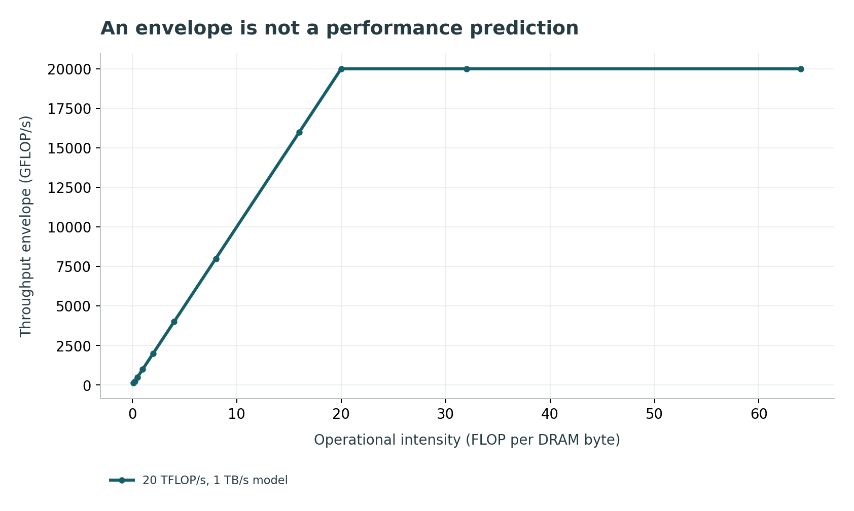
Assumptions: One precision and operation-count convention; No launch, instruction or occupancy bottleneck

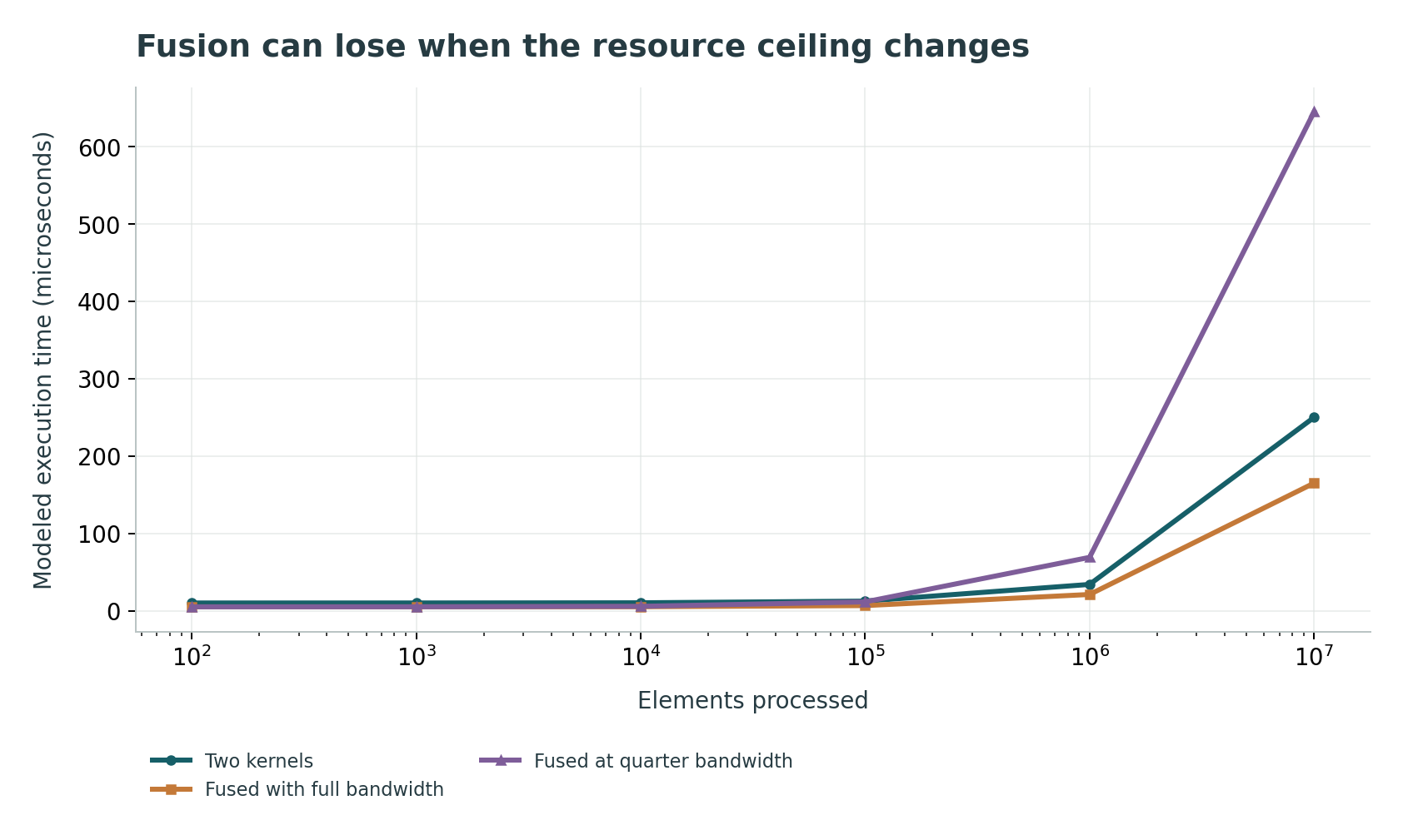
Assumptions: 5 us launch per kernel; no overlap; Separate 4N FLOPs / 24N bytes; fused 6N FLOPs / 16N bytes; Constrained fused bandwidth 250 GB/s is an assumption

Executed finite checks
2 check groups passed. The listed cases validate this model; they are not independent experiments or system benchmarks.
- Units and ridge-point consistency · 3 cases. 20,000 GF/s divided by 1,000 GB/s gives 20 FLOP/byte; intensity 0.125 bounds throughput at 125 GF/s.
- Fusion benefit and resource-loss counterexample · 4 cases. At N=1e6, separate kernels take 34 microseconds versus 21 for ideal fusion and 69 for constrained fusion. The crossover is 125,000 elements.
Comparison
| Quantity | What it describes | What it cannot establish alone |
|---|---|---|
| Occupancy | Resident active warps relative to device maximum | Throughput or useful work |
| Operational intensity | Operations per byte at a declared boundary | Attainable issue rate |
| Kernel time | One execution interval under stated measurement | End-to-end application speed |
| Profiler counters | Behavior under a collection method | Uninstrumented elapsed time |
| Correctness tolerance | Accepted numerical deviation | Performance across all input shapes |
Proposed validation protocol
- Fix the mathematical task, precision and acceptance tolerance.
- Record source, compiler, driver and documentation revisions.
- Define the workload shape distribution and weighting objective.
- Measure unprofiled end-to-end and kernel intervals separately.
- Calibrate relevant compute and memory ceilings under matching conditions.
- State a mechanism-specific hypothesis before each change.
- Collect targeted counters with the replay mode recorded.
- Test numerical edge cases and shape boundaries.
- Report cold/warm behavior and autotuning amortization.
- Publish both favorable and unfavorable regions with uncertainty.
Limitations
- Synthetic resource ceilings do not predict any commercial GPU.
- The fusion model assumes no overlap and fixed launch costs.
- The lower-bandwidth fused variant is a counterexample assumption, not an observed effect.
- No hardware kernel or numerical accuracy experiment was run for this article.
- Official documentation is a living source; the access date is recorded.
- Historical occupancy examples demonstrate nonmonotonicity, not modern speedup values.
Open research questions
- Can a tuning policy predict when fusion changes the limiting resource before compiling every candidate?
- How should end-to-end numerical error constraints guide mixed-precision performance optimization?
- Which minimal counter set best distinguishes latency hiding, memory traffic and instruction bottlenecks without excessive measurement perturbation?
Evidence and its boundaries
- [1] Roofline connects operation intensity and resource ceilings.
- A bound does not assert attainability. Inspected: UCB/EECS-2008-134, Section 3 and operational-intensity definition.
- [2] Occupancy depends on register/shared-memory resources and is not monotonically related to performance.
- Device-dependent allocation details must be checked for the target. Inspected: CUDA Best Practices Guide Sections 11.1 and 11.3 inspected.
- [3] Metric collection can involve replay and execution overhead.
- Instrumented execution is not automatically baseline timing. Inspected: Nsight Compute Profiling Guide: Metric Collection and Replay.
- [4] Tiled GEMM coordinates storage, reuse and pipelining.
- Documentation does not prove every larger tile is faster. Inspected: CUTLASS Efficient GEMM: Software Pipelining and hierarchical tiling.
- [5] Instruction-level parallelism provides historical counterexamples to maximizing occupancy.
- 2010 devices and rates are not current hardware claims. Inspected: Volkov GTC 2010 slides 3–14 inspected.
- [6] Roofline analysis requires consistent time, operations and traffic and can use empirical ceilings.
- Calibration microkernels do not guarantee application attainability. Inspected: NERSC Roofline Performance Model: empirical ceilings and intensity.
References
- Roofline: An Insightful Visual Performance Model for Floating-Point Programs and Multicore Architectures
Samuel Webb Williams, Andrew Waterman, David A. Patterson. University of California, Berkeley, UCB/EECS-2008-134 (2008). https://www2.eecs.berkeley.edu/Pubs/TechRpts/2008/EECS-2008-134.pdfSource access and scope
Report metadata and selected model definition inspected; distinguished from the 2009 CACM publication.
- CUDA C++ Best Practices Guide
NVIDIA. NVIDIA Documentation (2026). https://docs.nvidia.com/cuda/cuda-c-best-practices-guide/Source access and scope
Living documentation accessed 2026-10-25; version 13.4 displayed. Occupancy and execution configuration sections inspected. Year is access year, not an asserted original publication year.
- Nsight Compute Profiling Guide
NVIDIA. NVIDIA Documentation (2026). https://docs.nvidia.com/nsight-compute/ProfilingGuide/index.htmlSource access and scope
Living documentation accessed 2026-10-25; metric collection, replay and overhead descriptions inspected. Year denotes access.
- Efficient GEMM in CUDA
NVIDIA. CUTLASS Documentation (2026). https://docs.nvidia.com/cutlass/latest/media/docs/cpp/efficient_gemm.htmlSource access and scope
Living documentation accessed 2026-10-25; tiling and software-pipelining sections inspected. Year denotes access.
- Better Performance at Lower Occupancy
Vasily Volkov. GPU Technology Conference (2010). https://www.nvidia.com/content/GTC-2010/pdfs/2238_GTC2010.pdfSource access and scope
Title/date and selected slides 3–14 inspected; historical hardware examples not reproduced.
- Roofline Performance Model
NERSC. NERSC Documentation (2026). https://docs.nersc.gov/tools/performance/roofline/Source access and scope
Living official documentation accessed 2026-10-25; model, empirical ceilings and intensity sections inspected. Year denotes access.