
Skew Is the Workload: Partitioning and Direction Choice in Graph Processing
Exact graph counterexamples reveal why partition balance, traversal direction, and pipeline costs must be studied together.
English original. Translations of this new review are not yet available.
Abstract
Graph size alone does not characterize graph-processing work. Degree concentration, diameter, frontier composition, neighbor order, and state placement can change both the number of operations and their distribution across workers. This analytical review connects six primary sources on PowerGraph, direction-optimizing BFS, Ligra, GraphX, GraphIt, and Graph 500 methodology to argue for joint evaluation of partitioning and traversal direction. Reproducible standard-library models use stars, paths, and cliques as exact structural examples. A 64-vertex star gives equal vertex counts but a maximum worker load approximately 2.476 times the average. A constructed clique frontier demonstrates early-exit savings, while an endpoint search on a 64-vertex path supplies a counterexample to unconditional pull traversal: 3907 adjacency probes versus 126 for push. These values are analytical operation counts, not measured speedups. The review separates ideal task balance from replication cost, frontier conversion from edge work, normalized benchmark rates from actual probes, and kernel time from pipeline time. A proposed evaluation protocol records per-round work and communication under matched resource limits and independent correctness checks. The resulting research agenda seeks affordable predictors of the best feasible schedule while making workload scope and optimization costs explicit.
In this paper
- The graph is not a uniform bag of edges
- Vertex balance can hide edge imbalance
- Splitting a hub creates a state problem
- Push and pull perform different work
- A clique gives an exact early-exit example
- A path defeats unconditional pull
- Frontier representation belongs in the budget
- Locality and parallelism can pull in opposite directions
- The pipeline can dominate the kernel
- Normalized edge rate is not actual probe rate
- A joint partition-and-direction experiment
- The boundary of a structural explanation
The graph is not a uniform bag of edges
Two graphs with the same numbers of vertices and edges can impose very different workloads. Degree concentration changes which workers receive expensive vertices. Diameter changes how many traversal rounds occur. Community structure changes communication, while the active frontier changes which part of the graph matters at a particular moment. A performance claim that names only graph size leaves out variables that can determine the algorithmic work itself.
PowerGraph's discussion of natural graphs motivates treating degree skew as a structural challenge to placement and vertex computation. This review develops that insight alongside direction-optimizing BFS, Ligra, GraphX, GraphIt, and the Graph 500 specification. Its thesis is that partitioning and traversal direction should be evaluated jointly against the evolving active workload. A balanced static representation can still create an imbalanced round; a direction that reduces adjacency probes can still lose after representation conversion or communication. The accompanying models use small stars, paths, and cliques because their behavior is exactly inspectable. These are counterexample generators and accounting illustrations, not surrogates for measured distributed-system performance or empirical claims about the frequency of particular graph structures.
Sources [1]
Vertex balance can hide edge imbalance
Consider an undirected star with 64 vertices, represented by two directed adjacency entries for each of its 63 edges. Assign vertex identifiers modulo four to four workers, with the hub numbered zero. Every worker owns sixteen vertices. The hub's worker nevertheless owns 78 adjacency entries: 63 from the hub and one from each of fifteen leaves. The average is only 31.5, giving a maximum-to-average work ratio of 2.4761904762 under unit cost per entry.
An ideal distribution of the 126 directed edge tasks would have a maximum of 32 per worker. Figure one compares these quantities for stars of several sizes. The ideal curve is a lower bound on task balance and omits the cost of replicating or coordinating vertex state; it is not a runnable edge-partitioning implementation. The example refutes the proposition that equal vertex counts imply balanced graph work. It also identifies why an average degree is insufficient: the hub's indivisible adjacency scan creates a local lower bound unless the execution model can split it. A partitioning report should therefore include the largest assigned degree mass and active work per round, not just the number of vertices stored on each machine.
Splitting a hub creates a state problem
Factoring work across edges can reduce the concentration created by a high-degree vertex, but the vertex's state must then be read, updated, or aggregated across the participating partitions. A decomposition is easy when contributions can be combined under an associative operation and the consistency rule permits the required order. It is more complicated when updates depend on sequence, involve floating-point reductions with reproducibility requirements, or modify shared neighboring state.
The star model intentionally avoids these issues by counting edge tasks only. An implementation study should add the number of replicated vertex copies, synchronization messages, bytes transferred, and critical-path reduction depth. A hub spread across every worker may balance scans while creating a communication bottleneck at reconciliation. Conversely, keeping it local can be beneficial when its state is large and its edges are rarely active. The important quantity is the cost of the complete program step, not the visual evenness of an edge partition. A useful contract should specify whether results require bitwise reproducibility, mathematical equivalence under reassociation, or tolerance-bounded numerical agreement. Partitioning cannot be judged independently of the semantics of the aggregation it enables.
Push and pull perform different work
Direction-optimizing BFS uses an asymmetry in the search problem. A push step examines outgoing edges from the current frontier to discover unvisited vertices. A pull step examines incoming neighbors of each unvisited vertex and can stop as soon as it finds any frontier parent. Beamer and colleagues explicitly combine these approaches because pull's early exit is valuable in some frontier regimes and wasteful in others. The original discussion also identifies representation conversion and directed-graph storage implications.
The constructed probe count follows that same narrow BFS logic. It does not generalize early exit to algorithms that must aggregate every neighbor contribution. For example, a sum of all incoming values cannot stop after one match without changing the computation. Even for BFS, pull's work depends on neighbor order and the fraction of neighbors in the frontier. The associated cost model should therefore distinguish a semantic permission to stop from a probabilistic expectation of stopping early. This distinction is central to comparing frameworks: two implementations can both call an operation pull while performing different amounts of work because one uses a valid early-exit condition and the other must inspect every relevant neighbor.
Sources [2]
A clique gives an exact early-exit example
Take a complete undirected graph on 32 vertices and a frontier consisting of the first sixteen identifiers. Assume those frontier vertices are already visited and the remaining vertices are unvisited. In one constructed step, push inspects 16 times 31, or 496, adjacency entries. Pull inspects sixteen entries in total because each remaining vertex encounters vertex zero, a frontier member, first in its canonical neighbor order. Both discover the same remaining vertices.
Figure two varies the frontier size while retaining this ordering rule. The formulas are exact for the declared one-step state, and the implementation checks them by enumerating adjacency lists. The state is an analytical frontier scenario, not a claim about the intermediate state of ordinary single-source BFS on a clique, whose search completes differently. That boundary matters: a convenient frontier can demonstrate a mechanism without representing a complete execution trace. The example establishes how large redundant push work can be when many frontier edges lead to already visited vertices or share the same destination. It does not establish a runtime speedup of 31 times, because vertex scanning, memory access, bitmap lookup, and parallel scheduling remain outside the probe count.
A path defeats unconditional pull
Now use a path with 64 vertices and start BFS at one endpoint. The frontier contains essentially one vertex per level. Push traverses 126 adjacency entries across the complete search, once for each directed representation of an undirected edge. Always using pull performs 3907 adjacency probes with the model's canonical neighbor order, repeatedly scanning vertices that remain far from the frontier. The resulting distance maps agree exactly.
This is a direct counterexample to treating pull as an unconditional optimization. The model checks agreement for both push and pull over 64 explicit graphs: stars and paths with sizes two through thirty-three. That finite family verifies the two implementations on structurally distinct examples, but it is not a proof of their correctness on arbitrary graphs. The path also shows why a benchmark dominated by low-diameter graphs may favor a direction policy that is poorly suited to a different application. Workload selection should include high-diameter and disconnected cases, with source vertices chosen under a stated rule. Reporting only the fastest search root can hide the regime in which the policy makes its most expensive mistake.
Frontier representation belongs in the budget
Ligra exposes vertex subsets and edge operations while switching between sparse and dense representations. Its original description makes clear that representation and traversal order are connected choices. A sparse list is convenient for visiting a small frontier, whereas a dense representation supports fast membership tests across a broad scan. Conversion and duplicate elimination can add work that a count of adjacency probes does not capture.
A proposed direction controller should charge for constructing, clearing, and converting frontier data structures, including the cost of resetting state between searches. If a bitmap must be cleared over every vertex, sparse workloads may pay a graph-wide cost despite touching few edges. Generation counters or sparse clearing can alter that balance, but they carry their own memory and overflow considerations. The model deliberately uses Python sets so that its correctness and probe accounting remain simple; its runtime is not a proxy for an optimized bitmap implementation. An empirical study should measure total time and conversion time separately, then compare the selected schedule with an oracle constrained to the same representation costs. A free-conversion oracle would exaggerate the opportunity available to a practical controller.
Sources [3]
Locality and parallelism can pull in opposite directions
GraphIt's separation of algorithm and schedule makes traversal direction, layout, parallelization, and other execution choices explicit. The paper frames these choices through competing concerns including locality, parallelism, and work efficiency. This is useful evidence against ranking one scheduling technique without considering its composition with the others. A schedule that reduces logical work may expose fewer independent tasks or worsen the locality of the remaining accesses.
For the present analysis, suppose splitting a high-degree adjacency list improves worker balance but scatters accesses to destination state. The operation count falls on the critical worker while remote memory traffic rises. Alternatively, batching destinations may improve locality while delaying updates or increasing temporary storage. The best combination depends on the graph, algorithm, machine topology, and active set. A verification protocol should therefore vary schedules with algorithm semantics held constant and include correctness checks after each composition. It should also charge an autotuner for its search budget and report whether tuning data overlaps evaluation graphs. A schedule selected after observing every test outcome is an oracle comparison, not evidence that a deployed controller can make the same choice online.
Sources [5]
The pipeline can dominate the kernel
GraphX's author manuscript argues for combining graph-parallel and data-parallel operations, motivated by the cost and complexity of moving between specialized systems during an analytics pipeline. Its abstract supports the claim that graph construction, transformation, and computation deserve a common evaluation boundary. This review does not reproduce its performance results or infer the cost of specific current implementations from the preprint.
Consider a pipeline that filters records, builds a graph, runs several searches, and joins the answers back to source attributes. A faster BFS kernel may not improve end-to-end completion if graph materialization or transfer dominates. Reusing a preprocessed graph can be appropriate for repeated analytics, but then the amortization assumption should be explicit. For one-shot analysis, construction and conversion must remain visible. Updates create another distinction: a partition that is attractive for a static graph may be expensive to maintain as edges arrive or disappear. A complete experiment should report build time, storage expansion, update cost, kernel time, and output integration separately. That decomposition lets readers transfer the result to workloads with different reuse counts instead of treating one normalized kernel score as a universal pipeline ranking.
Sources [4]
Normalized edge rate is not actual probe rate
The Graph 500 specification defines validation rules, timing boundaries, and a normalized traversed-edges-per-second metric based on edges in the searched component. The numerator is a benchmark convention: the cited specification counts undirected edges in the traversed component using its self-loop and halved non-self-loop tuple rule. It should not be confused with the exact number of adjacency probes an optimized algorithm executes. A direction-optimizing traversal can increase the normalized rate precisely by avoiding redundant probes, not by making the hardware perform every original probe faster.
For interpretation, report both normalized throughput and actual work when instrumentation permits. Also report wall time, peak memory, preprocessing, and communication. An apparent superlinear speedup can reflect a change in work or cache behavior rather than an impossible increase in per-core processing rate. Correctness validation must remain independent of the performance metric. Small graphs can be compared against a reference distance computation, while large experiments may require structural checks that establish valid parent relationships and distances under the chosen benchmark. The specification's exclusion of validation from timed search is a declared boundary, not permission to omit validation altogether. A research report should preserve that distinction and avoid presenting compliance with a timing convention as evidence that a result was actually checked.
Sources [6]
A joint partition-and-direction experiment
The central hypothesis is that policies based only on static degree balance or frontier size will mispredict performance when active degree mass, neighbor ordering, and communication vary independently. A controlled study should include stars, paths, community graphs, and generated skewed graphs alongside appropriately licensed real datasets. Keep graph semantics, directionality, duplicate-edge handling, and source selection fixed across implementations. Record graph construction and any inverse-adjacency creation before timing the declared kernel boundary.
At every round, collect frontier vertices, frontier degree mass, unvisited degree mass, actual probes, worker imbalance, conversion cost, and transferred bytes. Compare static push, static pull, a declared hybrid heuristic, and an offline direction oracle with the same representation constraints. Repeat across partition policies and machine counts while preserving memory limits. Validate distances or other algorithm-specific invariants after each run. The hypothesis fails if the additional workload features do not improve predictions outside the tuning set, or if collecting them costs more than the scheduling improvement saves. This protocol makes adaptation accountable: a controller must select a better complete execution, not merely explain after the fact why one direction happened to win.
The boundary of a structural explanation
The models establish exact adjacency-work counts for the authored graphs and frontier states, demonstrate that vertex-count balance can conceal a hub bottleneck, and verify push-pull distance agreement over a finite test family. They do not measure distributed communication, NUMA behavior, GPU occupancy, or framework overhead. The ideal edge-balance curve is explicitly a lower bound rather than a realizable zero-cost partition. These limits are essential to the manuscript's claim of reproducibility: a reader can reproduce what was calculated without being invited to mistake it for what was measured.
The broader conclusion is that skew should enter the workload description at the level where the program spends work. Static degrees are one component; active-frontier composition, repeated scans, state replication, and data movement are others. A useful graph benchmark preserves enough of these dimensions to explain why a scheduling choice succeeds or fails. The next research step is to identify inexpensive observations that predict changes in the best feasible schedule before the expensive round begins. Such a predictor would connect structural understanding to a falsifiable systems contribution, while retaining correctness and complete cost accounting as constraints on every optimization.
Mathematical model
(1) Unit adjacency work for vertex owner pi, p workers and directed adjacency entries E_d; I excludes communication and state costs.
(2) Exact adjacency probes for the declared push step that scans every outgoing edge in frontier F, regardless of visited status.
(3) For vertices with a matching frontier neighbor, count through the first match; use full degree when none exists. U is the unvisited set.
(4) Constructed n-vertex clique with frontier vertices 0 through f-1 and canonical neighbor order; one-step state, not a complete single-source BFS trace.
(5) Illustrative time model: r_j is work rate and C_j communication time. It assumes serialized local computation and communication, a barrier and separate conversion; overlap and contention invalidate this approximation.
(6) Graph 500 normalized rate uses its undirected component-edge count m (self-loop tuples plus half the non-self-loop tuple count) and declared search time; it is not actual directed adjacency-probe rate.
Reproducible analytical figures
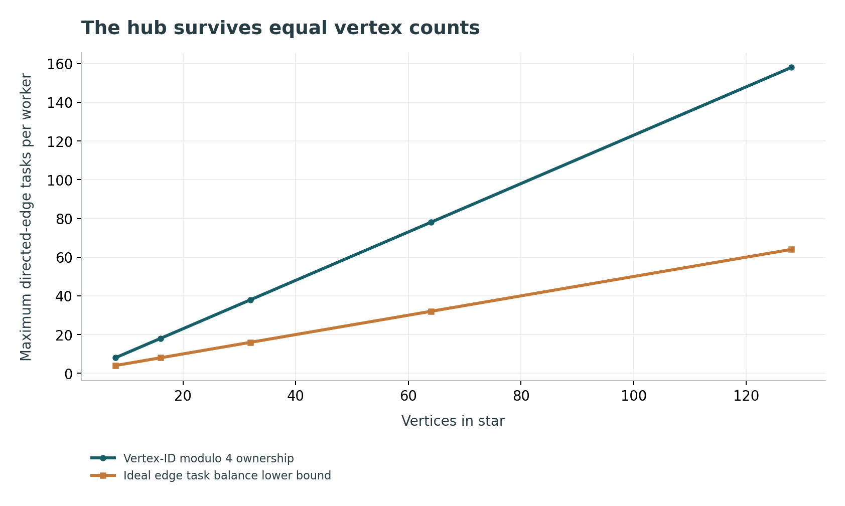
Assumptions: Four workers; Unit cost per adjacency entry; No communication or memory contention

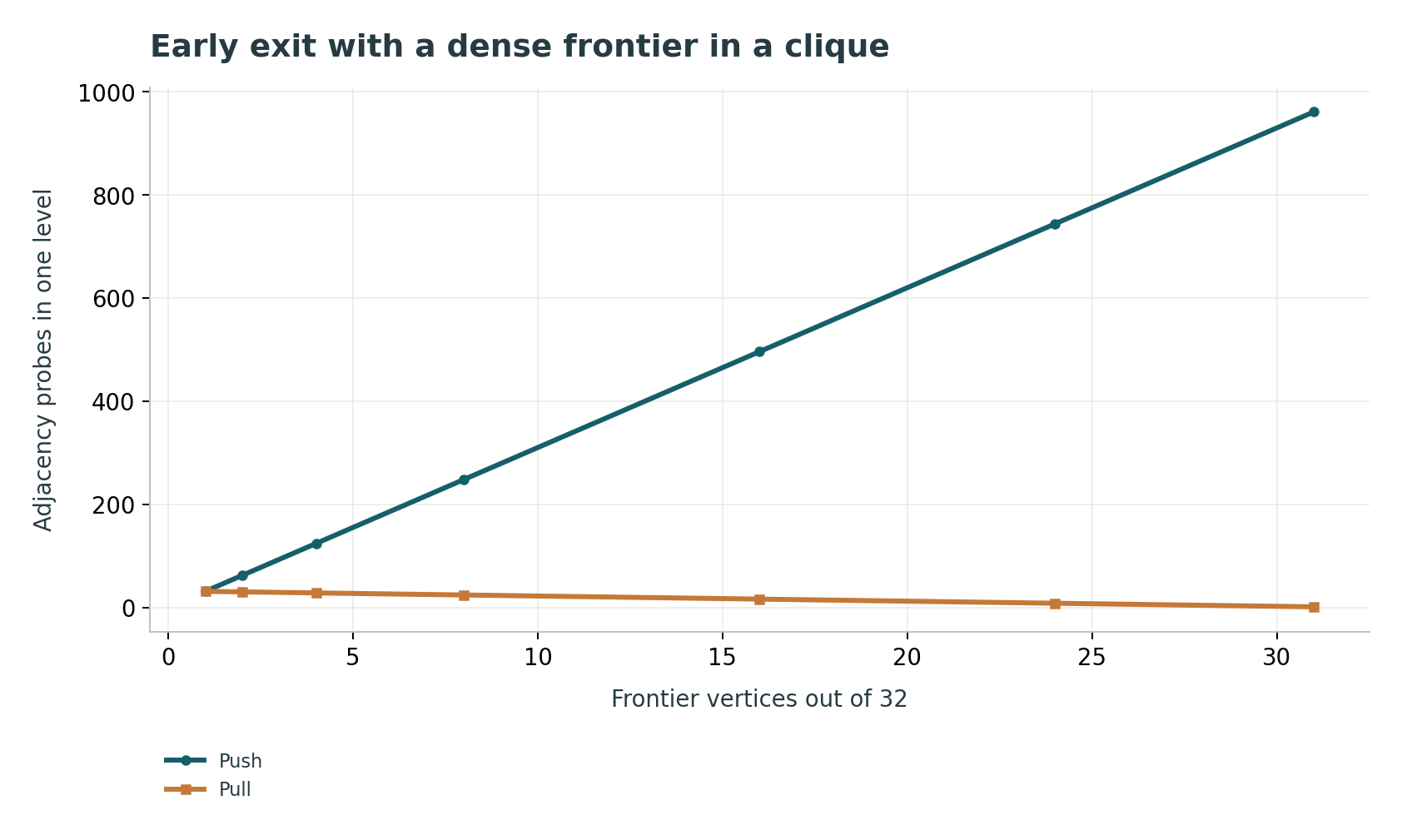
Assumptions: Exact BFS step semantics; Frontier is vertices 0 through f-1; No frontier-format conversion overhead

Executed finite checks
5 check groups passed. The listed cases validate this model; they are not independent experiments or system benchmarks.
- Push and pull recover identical BFS distances · 64 cases. 64 explicit connected graphs, canonical neighbor order.
- Closed-form distances independently validate both traversals · 64 cases. Known star/path distance formulas provide an oracle independent of push-pull agreement.
- Path is a counterexample to unconditional pull · 1 cases. Pull scans undiscovered vertices repeatedly on a high-diameter path.
- Complete-graph single-step probe formulas · 7 cases. Exact enumeration independently checks frontier degree and early-exit formulas.
- Vertex balance can hide edge imbalance · 1 cases. 64-vertex star; four equal vertex-count partitions.
Comparison
| Constructed case | Push or vertex-owned work | Pull or ideal work | Meaning |
|---|---|---|---|
| 64-vertex star, four workers | Maximum 78 entries | Ideal maximum at least 32 | Balance lower bound omits replication |
| 32-vertex clique, frontier 16 | 496 probes | 16 probes | One-step ordered-neighbor example |
| 64-vertex path, endpoint BFS | 126 probes | 3907 probes | Always-pull counterexample |
Proposed validation protocol
- Pin graph semantics, source vertices, framework versions and machine topology.
- Include graph families varying degree skew, diameter and community structure independently.
- Measure construction, partitioning and inverse-adjacency costs separately.
- Validate small outputs against an independent reference traversal.
- Compare vertex ownership and edge task distributions with equal memory budgets.
- Evaluate static push, static pull, a declared hybrid and a constrained oracle.
- Record per-round frontier size, degree mass, probes, imbalance and communication.
- Charge frontier conversion and online decision overhead to the selected schedule.
- Report normalized throughput alongside time, actual work and peak memory.
- Evaluate held-out graphs and include failed or resource-exhausted runs.
Limitations
- Models count adjacency probes, not elapsed execution time.
- Ideal edge task balance omits vertex replication and reconciliation.
- Clique frontier states are analytical scenarios rather than natural single-source BFS levels.
- Finite graph-family agreement is not a general correctness proof.
- No parallel runtime, NUMA, GPU or network experiment was executed.
- GraphX access is to the specified author preprint abstract, not a full implementation audit.
Open research questions
- Which inexpensive frontier statistics predict when direction changes repay conversion and communication?
- How should partitioning adapt when the active degree distribution differs from the stored graph?
- When does reducing kernel work improve complete graph-analytics pipelines after construction and update costs?
Evidence and its boundaries
- [1] Skewed degree distributions challenge graph-parallel placement and motivate factoring vertex work across edges.
- The review does not reproduce PowerGraph鈥檚 distributed experiments or all consistency strategies. Inspected: USENIX abstract; paper Sections 3 and 4 via indexed original text.
- [2] Bottom-up BFS can stop after finding a parent, and combining directions avoids its poor sparse-frontier behavior.
- Probe reductions do not directly imply equal runtime speedups; hardware results are not reproduced. Inspected: Sections IV and V.
- [3] Sparse and dense frontier representations support different edge-traversal choices in shared memory.
- No claim of distributed-memory equivalence or reproduced Ligra benchmark. Inspected: Introduction; vertexSubset and edgeMap descriptions.
- [4] GraphX unifies graph and data-parallel operations to reduce pipeline composition costs.
- Abstract-only review does not establish implementation-specific join rules or performance portability. Inspected: Abstract and submission record.
- [5] Separating algorithm from schedule exposes direction, layout and parallelization choices for composition.
- No compiler validity proof or performance experiment was independently reproduced. Inspected: Abstract; Section 4.
- [6] The benchmark defines correctness validation, timing boundaries and a normalized TEPS numerator.
- Specification version 2.0 dated 2017; accessed page is not a benchmark run or current ranking. Inspected: Sections 8, 9.1 and 9.2.
References
- PowerGraph: Distributed Graph-Parallel Computation on Natural Graphs
Joseph E. Gonzalez, Yucheng Low, Haijie Gu, Danny Bickson, Carlos Guestrin. USENIX OSDI (2012). https://www.usenix.org/conference/osdi12/technical-sessions/presentation/gonzalezSource access and scope
Original USENIX abstract and bibliography; indexed original paper discussion of degree skew and decomposition.
- Direction-Optimizing Breadth-First Search
Scott Beamer, Krste Asanović, David Patterson. SC (2012). https://people.eecs.berkeley.edu/~krste/papers/beamer-sc2012.pdfSource access and scope
Author-hosted original PDF abstract and Sections IV-V, including bottom-up algorithm and hybrid direction discussion.
- Ligra: A Lightweight Graph Processing Framework for Shared Memory
Julian Shun, Guy E. Blelloch. ACM PPoPP (2013). https://jshun.csail.mit.edu/ligra.pdfSource access and scope
Original author-hosted PDF abstract and sparse/dense vertexSubset and edgeMap descriptions.
- GraphX: Unifying Data-Parallel and Graph-Parallel Analytics
Reynold S. Xin, Daniel Crankshaw, Ankur Dave, Joseph E. Gonzalez, Michael J. Franklin, Ion Stoica. arXiv author manuscript (2014). https://arxiv.org/abs/1402.2394Source access and scope
Original author-submitted record, complete author list and abstract; this exact preprint is cited rather than conflated with later conference author ordering.
- GraphIt: A High-Performance Graph DSL
Yunming Zhang, Mengjiao Yang, Riyadh Baghdadi, Shoaib Kamil, Julian Shun, Saman Amarasinghe. Proceedings of the ACM on Programming Languages (2018). https://commit.csail.mit.edu/papers/2018/graphit.pdf
DOI: 10.1145/3276491Source access and scope
Original author-hosted paper abstract and Section 4 scheduling-language passages.
- Graph 500 Benchmark Specification
David A. Bader, Jonathan Berry, Simon Kahan, Richard Murphy, Jeremiah Willcock, Anton Korzh, Marcin Zalewski. Graph 500 (2017). https://graph500.org/?page_id=12Source access and scope
Original specification contributor list and version history, validation and timing/TEPS sections.