
Data and Training Reliability / DEEP LEARNING III
Noisy Labels and the Missing Identification Assumption
A classifier trained on corrupted labels observes a distribution of inputs and reported outcomes.
English original. Translations of this new review are not yet available.

Abstract
A classifier trained on corrupted labels observes a distribution of inputs and reported outcomes. It does not directly observe the clean target distribution or the mechanism that changed the labels. Increasing model capacity can improve estimation of the observed distribution without resolving that missing information. This analytical review supplies exact constructed controls, explicit assumptions, and a proposed empirical evaluation; no neural benchmark is claimed.
In this paper
- 1. Better fitting does not identify the clean label
- 2. Primary studies make different assumptions
- 3. Write the observation process before choosing a loss
- 4. Two incompatible worlds can look identical
- 5. Knowing the transition matrix changes the problem
- 6. Inversion amplifies uncertainty near singularity
- 7. Anchor assumptions supply identifying structure
- 8. Instance-dependent noise changes what can be learned
- 9. Small loss is not synonymous with correct annotation
- 10. Robust losses change the influence function
- 11. A clean evaluation set is itself a measurement instrument
- 12. Data cleaning should preserve an audit trail
- 13. A test plan that can distinguish assumptions
- 14. What the executable constructions prove
- 15. The useful question is where identification comes from
- 16. Sampling uncertainty can be amplified even with known noise
1. Better fitting does not identify the clean label
A classifier trained on corrupted labels observes a distribution of inputs and reported outcomes. It does not directly observe the clean target distribution or the mechanism that changed the labels. Increasing model capacity can improve estimation of the observed distribution without resolving that missing information.
This review focuses on identifiability rather than ranking robust-training algorithms. In a binary construction, two different clean class probabilities and corruption mechanisms produce exactly the same observed positive-label probability. No amount of additional data from that same observation process can distinguish them without extra assumptions. A second calculation shows how inversion becomes sensitive as the corruption mechanism approaches a singular case. These examples do not claim that real datasets follow a constant class-conditional noise model. They show why a successful denoising method must obtain identifying information from somewhere: trusted labels, anchor conditions, multiple annotators, structural assumptions, or prior knowledge. The source of that information is part of the scientific claim.
2. Primary studies make different assumptions
Natarajan and colleagues study loss corrections for noisy labels. Scott, Blanchard, and Handy analyze asymmetric label noise and conditions supporting denoising. Patrini and colleagues develop loss-correction methods for deep networks under a class-dependent corruption model.
Northcutt, Jiang, and Chuang examine confident learning and estimation of label quality. Han and colleagues use co-teaching, where two networks select examples for one another. Zhang and Sabuncu study generalized cross-entropy losses for noisy-label training. These are distinct strategies with different assumptions and empirical scopes. Their inspected primary abstracts motivate the questions discussed here; they do not establish that every label error is identifiable or that one method dominates all corruption processes. We do not reproduce their reported benchmark results. Our calculations isolate a binary observation model and its inversion, providing an exact diagnostic for overbroad interpretations of label correction.
3. Write the observation process before choosing a loss
Let Y be a clean binary label and Y_tilde the observed label. Define a=P(Y_tilde=1|Y=0) and b=P(Y_tilde=0|Y=1). Under class-conditional noise independent of X given Y, the observed positive probability at input x is q(x)=a+(1-a-b)p(x), where p(x)=P(Y=1|X=x).
This relation is an assumption about the data-generation process, not a universal description of annotation errors. In many tasks, mistakes depend on image ambiguity, language, annotator expertise, or subpopulation, so a and b vary with x or other hidden variables. Even the concept of one clean label can be questionable for inherently ambiguous examples. A useful dataset study distinguishes factual mistakes, category-definition disputes, and legitimate uncertainty. Choosing a robust loss before defining which problem is being solved can produce a model that suppresses difficult but valid examples. The statistical model should therefore be justified with annotation evidence, not merely selected because its equations are convenient.
4. Two incompatible worlds can look identical
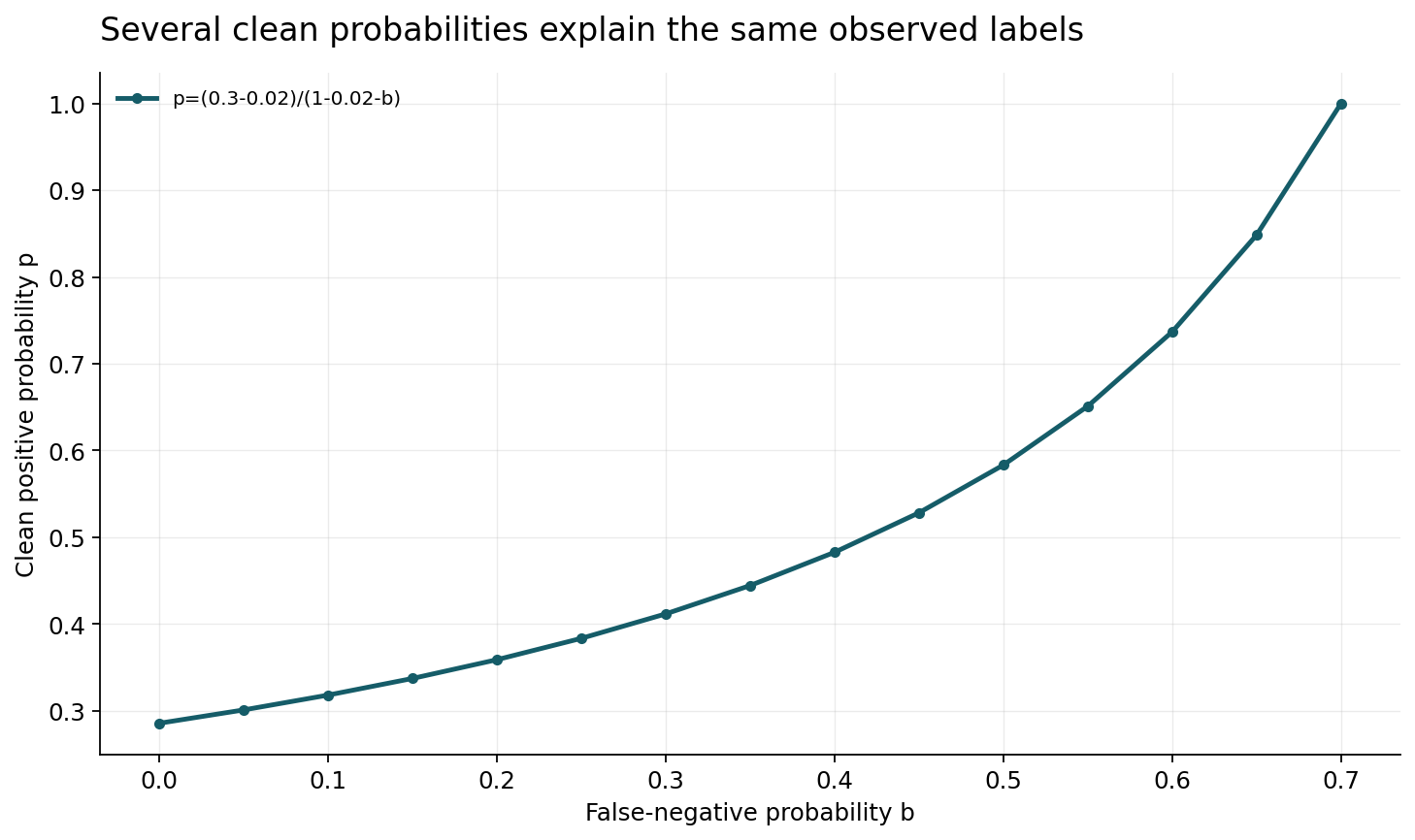
Consider an input region with observed positive-label probability q=0.3. One possible world has no corruption and clean probability p=0.3. Another has a=0.1, b=0.5, and clean probability p=0.5. The formula gives 0.1+0.4 times 0.5=0.3, so the observed labels are distributed identically in both worlds.
The clean Bayes decision may differ under other choices of the same construction. For example, with a=0.02 and b=0.58, the same observed q=0.3 corresponds to p=0.7. A learner seeing only observed labels cannot determine whether the clean positive probability is 0.3 or 0.7. This is an identification failure, not a shortage of optimization steps. The first figure varies compatible noise parameters and plots the corresponding clean probability for a fixed observed q. Only parameter combinations yielding probabilities in [0,1] are included. The curve is a family of possible explanations, not an estimate of the corruption rate in any real corpus.
5. Knowing the transition matrix changes the problem
If a and b are known and 1-a-b is nonzero, the clean probability follows by inversion: p=(q-a)/(1-a-b). That algebra identifies p within the declared model. It does not explain how the transition probabilities were learned, whether they are constant across inputs, or how estimation uncertainty propagates.
A benchmark that supplies the true synthetic transition matrix grants information unavailable in many real datasets. Such a benchmark is useful for testing a correction algorithm under controlled assumptions, but it should not be presented as an end-to-end solution to discovering real annotation errors. A complete evaluation separates oracle-transition performance from estimated-transition performance and from model-misspecification tests. It also specifies whether the clean labels used to estimate the transition are independent of evaluation labels. Otherwise, apparent robustness can partly reflect access to privileged target information. The distinction is similar to separating an inverse problem from measurement of the forward operator: solving one does not automatically solve the other.
6. Inversion amplifies uncertainty near singularity
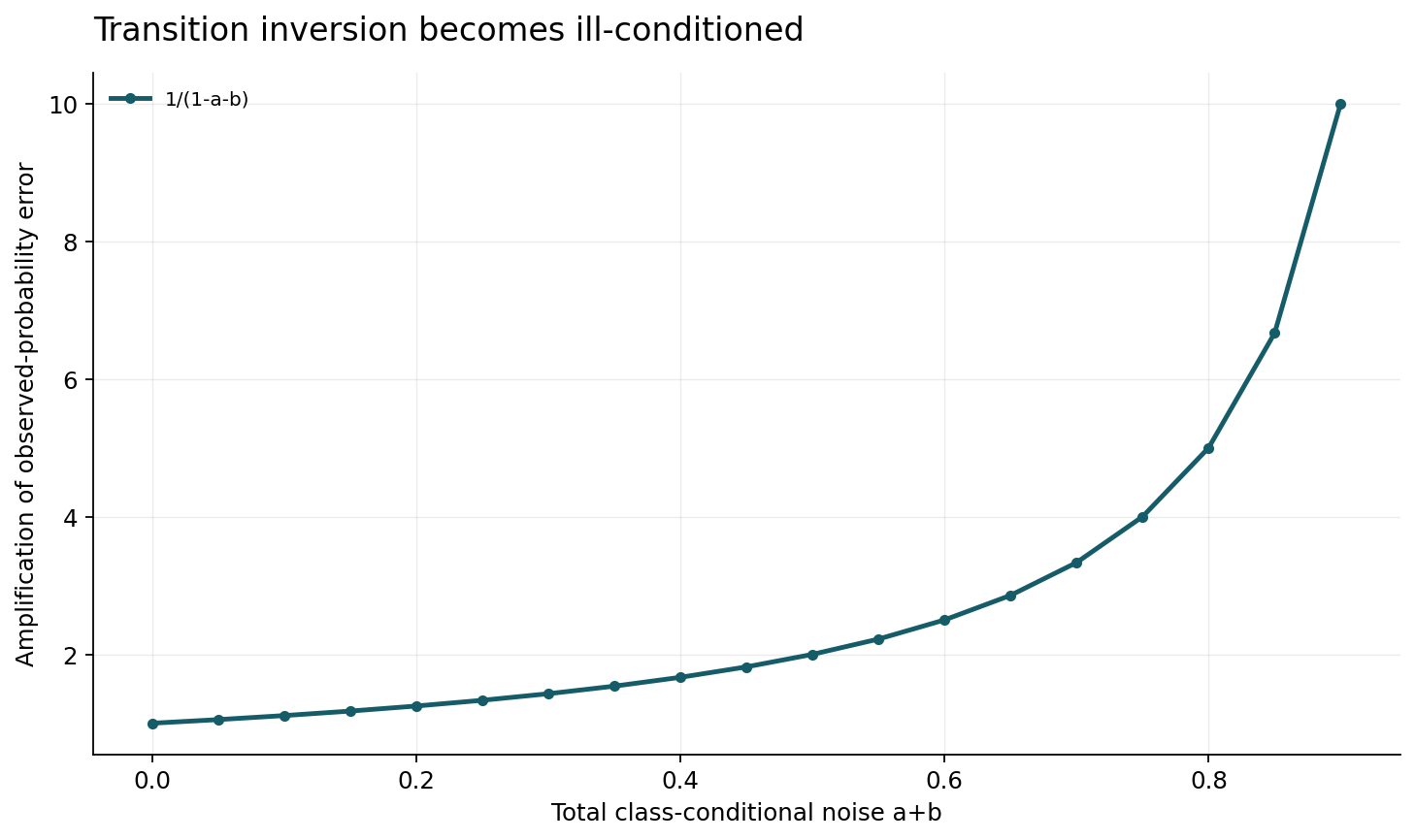
The derivative of p with respect to q is 1/(1-a-b). When a+b approaches one, small errors in observed probabilities can become large errors in the inferred clean probabilities. At a+b=1, q=a is independent of p and the labels contain no information about the clean class probability under this model.
The second figure shows the amplification factor for several total corruption levels below one. It is a deterministic conditioning calculation, not a measured generalization curve. Errors in a and b also matter, and their effects can be correlated with errors in q. Clipping an inverted estimate back into [0,1] enforces a valid probability range but does not restore lost information or remove bias. A report should therefore include uncertainty in the transition estimate and sensitivity to plausible alternatives. A mathematically invertible matrix can still be practically ill-conditioned. Treating inversion success as evidence of reliable denoising ignores the distinction between existence and stability.
7. Anchor assumptions supply identifying structure
One way to estimate corruption is to assume that some input regions have a clean class probability at or near zero or one. Under appropriate conditions, observed probabilities in those regions reveal parts of the transition mechanism. Such anchor assumptions are substantive claims about the data, not consequences of using a sufficiently expressive neural network.
A highly confident model prediction is not automatically an anchor point. The model may be confidently wrong, or its confidence may itself reflect the corrupted labels. To evaluate an anchor-based procedure, identify why the anchors are credible and test sensitivity when they are imperfect. Trusted annotations can help, but their sampling design matters: a clean subset containing only easy cases may not characterize noise on ambiguous cases. The practical question is whether the extra information breaks the nonidentifiability exhibited by the construction. If it does, the method should credit that information explicitly. If it does not, a precise estimate can still represent one arbitrary member of several observationally equivalent explanations.
8. Instance-dependent noise changes what can be learned
When a(x) and b(x) vary with the input, the observed q(x) has more unknown components. A single constant transition matrix may fit the average while being systematically wrong in important regions. A method can then improve overall accuracy yet worsen the very ambiguous cases where annotation quality is poorest.
This is not an argument against class-conditional models. They can be useful approximations or controlled testbeds. It is an argument for checking their adequacy. Stratify a trusted audit by difficulty, source, annotator, and relevant domain rather than sampling only uniformly. Compare conditional error patterns and preserve disagreement instead of forcing every case into a binary clean-or-noisy label. If multiple annotators are available, their dependence must be considered: several annotators copying the same source do not provide independent evidence. A credible noise model connects its assumptions to actual annotation practice, including how instructions, adjudication, and missing labels were handled.
9. Small loss is not synonymous with correct annotation
Many training heuristics treat low-loss examples as more likely to be clean. This can be useful early in some learning regimes, but it is not a logical equivalence. Easy systematic mislabels can have low loss, while rare valid patterns can remain high loss. A filtering policy can therefore reinforce the model's initial blind spots.
The evaluation should include controlled cases where a minority pattern is both valid and difficult, and cases where a repeated wrong label is easy to memorize. Measure which examples are discarded and how that changes population weights. If two models teach one another, their errors may still be correlated through shared architecture, training data, or initialization conventions. Agreement between them is evidence only relative to that dependence structure. A useful study separates noise detection precision, retained coverage, and final predictive performance. Improving one does not automatically improve the others. The binary identifiability example explains why a heuristic needs additional empirical support rather than a purely confidence-based claim of correctness.
10. Robust losses change the influence function
Replacing cross-entropy with another loss changes how strongly examples with different predicted probabilities affect training. A bounded or slowly growing loss can reduce the influence of extreme disagreements, but it may also reduce learning from legitimate hard examples. The tradeoff depends on the target and noise process.
One should distinguish robustness of an estimator under a specified contamination model from empirical tolerance of a particular synthetic corruption experiment. A method may have a useful theoretical property and still be poorly suited to another kind of label uncertainty. Loss normalization, class imbalance, and optimization budget also influence comparisons. Report the actual objective and gradient behavior rather than describing every reduced sensitivity as noise removal. A model can become less responsive to labels without identifying which labels are wrong. The right question is whether that reduced responsiveness improves the intended clean-data decision problem under assumptions supported by the dataset.
11. A clean evaluation set is itself a measurement instrument
Denoising experiments often rely on a supposedly clean test set. If that set contains annotation errors, model rankings can change for reasons unrelated to training robustness. Conversely, using the same examples to tune a noise detector and judge its success creates circular evidence.
A defensible evaluation documents how test labels were obtained, how disagreements were resolved, and which uncertainties remain. Some tasks require probabilistic or multi-annotator targets instead of one forced label. The evaluation metric should match that target. If human reannotation is performed only on examples where the candidate model disagrees with the benchmark, verification bias can favor the candidate. Use blinded, balanced sampling that includes agreements and disagreements from multiple models. Report corrected and original-label results separately rather than silently replacing the benchmark. This preserves comparability and makes clear whether an improvement comes from a better model, a revised measurement instrument, or both.
12. Data cleaning should preserve an audit trail
A label-cleaning pipeline should retain original labels, proposed corrections, confidence or rationale, reviewer identity where appropriate, and the version in which a correction became effective. Silent overwriting makes it impossible to determine what data produced a model or whether later evaluation used information unavailable at training time.
Automatic flags can prioritize review without being treated as definitive truth. The workflow should allow unresolved ambiguity, multiple valid labels, and reversal of an incorrect correction. For privacy-sensitive data, the audit can reference protected records without exposing them publicly. The scientific release should still report aggregate counts, sampling policies, and known limitations. Data cleaning changes the training distribution and can alter class prevalence, so downstream evaluation needs a new version boundary. An auditable process supports correction without pretending that the first machine-generated proposal was authoritative. This is especially important when the model that proposes corrections is later evaluated on the corrected dataset.
13. A test plan that can distinguish assumptions
Construct separate benchmark arms for known class-conditional noise, estimated class-conditional noise, and deliberately instance-dependent noise. Keep the clean evaluation set independent. Include oracle-transition correction as an upper-information control, ordinary training, robust-loss methods, and selection methods with matched model and compute budgets.
Report transition estimation error, noise-detection precision and recall, retained category coverage, clean predictive utility, and calibration where relevant. Vary class imbalance and hard-but-clean minorities. Test sensitivity to imperfect anchors and biased trusted subsets. Preserve all hyperparameter searches and failed runs. A method that wins only with an oracle transition is still informative, but the claim must identify that privilege. A method that remains useful under misspecification may deserve a different kind of empirical claim. The objective is to determine which source of identifying information supports each result, not to produce one ranking that erases differences in assumptions.
14. What the executable constructions prove
The program enumerates a finite grid of clean probabilities and corruption parameters, verifies the forward observation equation, and identifies distinct parameter triples with identical observed q but clean probabilities on opposite sides of one half. It checks inversion where the denominator is nonzero and verifies loss of identification at the singular boundary.
It also compares numerical perturbations in q with the analytical amplification factor, including zero-noise and near-singular controls. Figure arrays are generated from the same declared model and checked against independent algebraic identities. No neural network is trained, no labels are changed, and no real annotation error rate is estimated. The examples establish that observed predictive fit does not alone identify clean labels and that inversion can be unstable. They provide a compact way to challenge unjustified interpretations while leaving practical algorithm selection to appropriately controlled experiments.
15. The useful question is where identification comes from
Reliable noisy-label learning requires more than an optimizer that fits a modified loss. It requires a defensible account of the relationship between observed annotations and the intended target. That account may use trusted data, multiple observations, structural restrictions, or explicit uncertainty. Each choice supplies information and imposes limitations.
Open questions include how to audit those assumptions at scale, how to distinguish systematic mislabeling from legitimate ambiguity, and how to preserve rare valid examples during automatic cleaning. Another challenge is reporting uncertainty when transition estimation and predictive modeling share data and errors. The binary construction cannot solve these problems, but it shows why they cannot be ignored. A precise review should credit the assumptions that make denoising possible, test their failure modes, and avoid turning a model's confidence into an unearned claim about ground truth.
16. Sampling uncertainty can be amplified even with known noise
Assume for the moment that a and b are known exactly and that n independent observed labels are collected at one fixed input condition. The empirical positive frequency has variance q(1-q)/n. Before clipping to the probability interval, the inverted estimator has variance q(1-q)/[n(1-a-b)^2]. The squared denominator makes clear that near-singular corruption requires many more observations to obtain the same precision.
This is an elementary sampling calculation rather than a finite-sample guarantee for a neural classifier. A network estimates probabilities across inputs using shared structure, so bias, approximation, and dependence enter. Nevertheless, the calculation provides a useful lower-level sanity check: even a perfect knowledge of the transition matrix does not make weak observations informative. Increasing dataset size can reduce sampling variance, but it cannot resolve the exactly singular case where q no longer depends on p.
An estimated transition matrix introduces further uncertainty. Treating its entries as fixed after fitting can produce overly narrow intervals, especially if the same data also fit q. A proposed empirical study should use an appropriate joint uncertainty analysis or an independently held-out trusted sample, while reporting the design's limitations. A bootstrap must respect source or annotator dependence if those are the independent units.
The executable checks compare the variance expression with exact enumeration of a binomial count for a small n. This independent calculation validates the amplification mechanism without simulation noise. The boundary a=b=0 recovers ordinary Bernoulli estimation, and the near-singular cases show increasing variance as expected. The result supports a carefully bounded conclusion: identification and stable estimation are separate requirements, and satisfying the first does not automatically satisfy the second.
Core equations and definitions
(1) Binary class-conditional corruption.
(2) Identified only with known parameters and nonzero denominator.
(3) Conditioning of the inverse relation.
(4) Known noise parameters, independent Bernoulli labels, before probability clipping.
(5) Two observed-identical worlds with opposite clean Bayes decisions.
Constructed analytical figures
Comparison and reporting contract
| Choice | What changes | What must be checked |
|---|---|---|
| Known transition | Algebraic identification | Conditioning |
| Estimated transition | Additional uncertainty | Trusted data and anchors |
| Instance-dependent errors | More unknown functions | Adequacy of constant-noise assumptions |
Evaluation protocol
- Separate oracle and estimated transition arms.
- Keep clean test labels independent.
- Audit hard-clean and easy-noisy examples.
- Measure retention and uncertainty by justified strata.
Limitations
- Binary constant noise is a controlled model.
- No real labels are changed or audited.
- No neural training result is claimed.
Open research questions
- How can identifying assumptions be audited at scale?
- How should ambiguity differ from error?
- How can uncertainty in jointly estimated noise and prediction be propagated?
Evidence and its boundaries
- Loss correction can be studied under explicit label-corruption assumptions.
- [1] — Only the inspected abstract scope is asserted; no reproduction of source results. Inspected: Primary publisher or author arXiv abstract and metadata inspected via web on 2026-10-28; no independent proof or benchmark replication.
- Asymmetric denoising depends on identifying conditions.
- [2] — Only the inspected abstract scope is asserted; no reproduction of source results. Inspected: Primary publisher or author arXiv abstract and metadata inspected via web on 2026-10-28; no independent proof or benchmark replication.
- Deep loss correction uses a class-dependent corruption model.
- [3] — Only the inspected abstract scope is asserted; no reproduction of source results. Inspected: Official CVF primary abstract and bibliographic metadata inspected through indexed web search on 2026-10-28; direct page access returned HTTP 403. No full proof or benchmark replication.
- Confident learning estimates label quality under stated noise assumptions.
- [4] — Only the inspected abstract scope is asserted; no reproduction of source results. Inspected: Primary publisher or author arXiv abstract and metadata inspected via web on 2026-10-28; no independent proof or benchmark replication.
- Two networks select training examples for each other.
- [5] — Only the inspected abstract scope is asserted; no reproduction of source results. Inspected: Primary publisher or author arXiv abstract and metadata inspected via web on 2026-10-28; no independent proof or benchmark replication.
- Modified losses offer a different noisy-label training strategy.
- [6] — Only the inspected abstract scope is asserted; no reproduction of source results. Inspected: Primary publisher or author arXiv abstract and metadata inspected via web on 2026-10-28; no independent proof or benchmark replication.
References
- Learning with Noisy Labels
Nagarajan Natarajan, Inderjit S. Dhillon, Pradeep K. Ravikumar, Ambuj Tewari. Advances in Neural Information Processing Systems (2013). https://papers.nips.cc/paper_files/paper/2013/hash/3871bd64012152bfb53fdf04b401193f-Abstract.htmlSource scope
Primary publisher or author arXiv abstract and metadata inspected via web on 2026-10-28; no independent proof or benchmark replication.
- Classification with Asymmetric Label Noise: Consistency and Maximal Denoising
Clayton Scott, Gilles Blanchard, Gregory Handy. Proceedings of the 26th Annual Conference on Learning Theory (2013). https://proceedings.mlr.press/v30/Scott13.htmlSource scope
Primary publisher or author arXiv abstract and metadata inspected via web on 2026-10-28; no independent proof or benchmark replication.
- Making Deep Neural Networks Robust to Label Noise: A Loss Correction Approach
Giorgio Patrini, Alessandro Rozza, Aditya Krishna Menon, Richard Nock, Lizhen Qu. Proceedings of the IEEE Conference on Computer Vision and Pattern Recognition (CVPR) (2017). https://openaccess.thecvf.com/content_cvpr_2017/html/Patrini_Making_Deep_Neural_CVPR_2017_paper.htmlSource scope
Official CVF primary abstract and bibliographic metadata inspected through indexed web search on 2026-10-28; direct page access returned HTTP 403. No full proof or benchmark replication.
- Confident Learning: Estimating Uncertainty in Dataset Labels
Curtis G. Northcutt, Lu Jiang, Isaac L. Chuang. arXiv preprint (2019). https://arxiv.org/abs/1911.00068Source scope
Primary publisher or author arXiv abstract and metadata inspected via web on 2026-10-28; no independent proof or benchmark replication.
- Co-teaching: Robust Training of Deep Neural Networks with Extremely Noisy Labels
Bo Han, Quanming Yao, Xingrui Yu, Gang Niu, Miao Xu, Weihua Hu, Ivor W. Tsang, Masashi Sugiyama. arXiv preprint (2018). https://arxiv.org/abs/1804.06872Source scope
Primary publisher or author arXiv abstract and metadata inspected via web on 2026-10-28; no independent proof or benchmark replication.
- Generalized Cross Entropy Loss for Training Deep Neural Networks with Noisy Labels
Zhilu Zhang, Mert R. Sabuncu. arXiv preprint (2018). https://arxiv.org/abs/1805.07836Source scope
Primary publisher or author arXiv abstract and metadata inspected via web on 2026-10-28; no independent proof or benchmark replication.