
Data and Training Reliability / DEEP LEARNING III
Interpolation Changes the Learning Distribution
Mixing two training examples creates an additional input and a target assigned by a rule.
English original. Translations of this new review are not yet available.

Abstract
Mixing two training examples creates an additional input and a target assigned by a rule. That rule changes the distribution on which a predictor is optimized. It may encode a useful inductive preference, but it does not follow automatically from the original data-generating process. This analytical review supplies exact constructed controls, explicit assumptions, and a proposed empirical evaluation; no neural benchmark is claimed.
In this paper
- 1. Interpolation is a statistical intervention
- 2. The primary literature supports several mechanisms
- 3. Define the vicinal distribution explicitly
- 4. Two endpoints do not determine the correct interior
- 5. Classification accuracy can conceal probability mismatch
- 6. Mixing strength is not summarized by the mean weight
- 7. A quadratic expansion reveals an added constraint
- 8. Input geometry and semantic geometry can disagree
- 9. Hidden-state interpolation inherits a learned coordinate system
- 10. Spatial mixing uses a different label assumption
- 11. Calibration must be evaluated on the target distribution
- 12. Robustness claims need a specified perturbation set
- 13. Pairing policies can change class and source balance
- 14. A discriminating experimental design
- 15. Executable checks establish the limited analytical claims
- 16. Implications for interpretable augmentation research
1. Interpolation is a statistical intervention
Mixing two training examples creates an additional input and a target assigned by a rule. That rule changes the distribution on which a predictor is optimized. It may encode a useful inductive preference, but it does not follow automatically from the original data-generating process.
This review studies interpolation as a choice of training measure. A scalar construction compares a linear soft target between two labeled endpoints with a hard threshold target on the same interval. A second calculation isolates how uncertainty in mixing weights changes the strength of a midpoint penalty. Both are exact finite or analytical examples, not new image-classification experiments. They expose why statements such as smoother predictions or better calibration require a specified evaluation distribution. A model can be well matched to interpolated targets and still be biased relative to the actual task. The scientific question is when the chosen interpolation rule transfers useful structure to that task and how to test the boundary of that transfer.
2. The primary literature supports several mechanisms
Zhang and colleagues introduce mixup using convex combinations of inputs and labels. Verma and colleagues extend interpolation to hidden representations. Yun and colleagues study CutMix, which combines spatial regions with area-based targets rather than uniformly blending every input coordinate.
Zhang and colleagues analyze robustness and generalization effects, while related work studies when mixup improves calibration. Zou and colleagues investigate feature-learning benefits under specified models. These inspected primary records show that interpolation can influence representation, regularization, and confidence through different mechanisms. They do not establish that every convex combination has a physically meaningful soft label or that all tasks benefit. We use the original abstracts to identify these scopes and avoid importing source benchmark numbers. The constructions below are our own diagnostics for target mismatch and mixing strength, not reproductions of the cited experiments or proofs.
3. Define the vicinal distribution explicitly
Let (x_i,y_i) and (x_j,y_j) be two training examples and let lambda lie in [0,1]. Standard input mixing forms x_tilde=lambda x_i+(1-lambda)x_j and y_tilde=lambda y_i+(1-lambda)y_j. The training distribution now includes pairs and mixing weights, so it depends on pair selection, the distribution of lambda, and any restrictions on eligible examples.
A uniform pairing policy can mix across classes, domains, or sources that would never coexist in the intended population. A within-class policy encodes a different assumption. Using a symmetric beta distribution changes how often examples lie near endpoints or near the middle. These are part of the method, not interchangeable implementation choices. For categorical labels, a mixed target is a probability vector under the training objective. It should not be described as an observed empirical frequency unless independently justified. The interpolation rule provides supervision beyond the original labeled points, and that extra supervision is an assumption about desirable behavior between them.
4. Two endpoints do not determine the correct interior
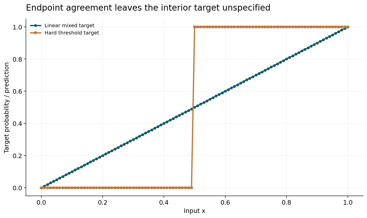
Consider x=0 with label zero and x=1 with label one. Linear interpolation assigns target t(x)=x throughout the interval. An alternative task has deterministic label h(x)=0 below one half and one above one half. Both agree at the endpoints, yet they disagree almost everywhere inside.
Under uniformly sampled x and squared probability error, the interpolated predictor f(x)=x has zero error against t but nonzero error against h. Integrating the two symmetric halves gives an error of 1/12. The hard-threshold predictor has zero error against h but the same nonzero discrepancy against t. Neither predictor is universally right: the evaluation target determines the answer. This is a deliberately simple counterexample to the claim that endpoint labels uniquely justify linear interior targets. It does not show that mixup is ineffective in real networks. It shows that interpolation introduces a prior whose suitability must be assessed with evidence about the task's geometry and uncertainty.
5. Classification accuracy can conceal probability mismatch
For the hard-threshold task, thresholding f(x)=x at one half yields the correct class almost everywhere, despite nonzero squared probability error. Thus a classifier can have perfect zero-one accuracy while its probabilities remain inappropriate for a deterministic target. Conversely, if t(x)=x represents the true conditional probability, a hard step is overconfident.
The first figure displays both target functions and the interpolation predictor on the same axis. A separate quantity reports the integrated discrepancy, with the target and measure explicitly stated. This distinction matters whenever calibration is used as an explanation for improved accuracy. Accuracy, proper scoring rules, and calibration assess different properties. A method can improve one while worsening another, especially under distribution shift. The constructed example uses a known uniform evaluation measure so the calculation is exact. Real evaluations need held-out data, uncertainty estimates, and a clear definition of which probabilities are being assessed.
6. Mixing strength is not summarized by the mean weight
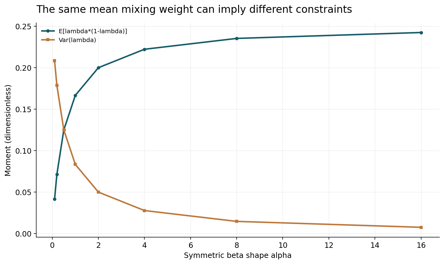
For lambda distributed as Beta(alpha,alpha), symmetry gives mean one half for every positive alpha. Yet the distribution ranges from endpoint-concentrated for small alpha to midpoint-concentrated for large alpha. The mean alone therefore fails to describe how strongly the algorithm constrains interior behavior.
A useful scalar is E[lambda(1-lambda)]=alpha/[2(2alpha+1)]. It approaches zero as alpha approaches zero and approaches one quarter as alpha grows. This quantity measures one form of interpolation leverage in quadratic constructions, not a universal regularization coefficient for arbitrary neural networks. The second figure plots it alongside the variance of lambda, which equals 1/[4(2alpha+1)]. Together they make the endpoint-versus-midpoint tradeoff explicit. A paper should report the actual sampling law and any transformations such as replacing lambda with max(lambda,1-lambda). Such transformations change the training measure even when an informal description still says beta mixup.
7. A quadratic expansion reveals an added constraint
For a linear predictor and squared loss, mixing inputs and targets mixes their residuals. If residuals are r_i and r_j, the mixed squared residual is lambda squared r_i squared plus (1-lambda) squared r_j squared plus 2lambda(1-lambda)r_i r_j. The cross term couples examples that were separate under ordinary empirical risk.
This identity explains why pair selection matters. Similar or opposing residuals interact differently, and the expected objective depends on how pairs are sampled. It also shows why a description of mixup as simply adding more independent data is incomplete. The additional examples are deterministic functions of existing observations and create structured constraints rather than new independent measurements. The expansion applies to the declared linear squared-loss setting; nonlinear networks and cross-entropy require different analyses. Its purpose is to supply an exact reference case against which broader intuitions can be tested. It should not be generalized into a universal claim that every interpolation method is equivalent to a particular parameter penalty.
8. Input geometry and semantic geometry can disagree
A convex combination in pixel space may not correspond to a plausible intermediate scene. Two speech waveforms can overlap acoustically without representing a meaningful halfway transcript. A mixture of two clinical records may violate physical or demographic constraints. Such examples do not make interpolation useless, but they challenge a literal semantic interpretation of the synthetic input.
The method can still act as a regularizer by specifying desired behavior off the observed manifold. That is a different claim from saying the synthetic example is a valid draw from the target population. A useful evaluation can distinguish on-manifold utility from off-manifold smoothness and test whether the imposed constraints interfere with rare valid cases. Pair restrictions or domain-aware transformations may improve relevance, but they add assumptions and tuning choices. The report should identify those choices rather than presenting the resulting data as naturally occurring observations. The analytical endpoint example is a minimal illustration of this gap between a coordinate operation and a scientific label model.
9. Hidden-state interpolation inherits a learned coordinate system
Interpolating hidden representations can avoid some obvious input artifacts, but it depends on the geometry learned by the encoder. Two semantically related examples need not lie on a meaningful straight path in that representation, and the geometry can change throughout training.
The layer chosen for mixing, whether gradients flow through both branches, and the pairing policy all affect the objective. A representation can make certain factors linear while entangling others. Therefore improved performance is evidence about the complete architecture and training procedure, not proof that the hidden space globally matches semantic geometry. Diagnostics can compare interpolation paths, class separation, and robustness across independently trained representations. They should also include tasks where linear interpolation is known to conflict with the target. Such negative controls make an explanation more informative than selecting only visually convincing examples. The scientific aim is to locate when the learned coordinate system supports useful constraints, not to assume that hidden means semantic.
10. Spatial mixing uses a different label assumption
Cut-and-paste augmentation preserves local image structure while replacing regions. Its target weight is often related to visible area, but area need not equal class evidence. A small object can occupy a tiny region while determining the label, and a pasted patch can remove that object entirely.
A careful implementation measures the actual clipped patch area after boundaries and resizing, rather than using a nominal sampled area. A careful scientific interpretation goes further: it asks whether the target mixture reflects the remaining semantic evidence. Object masks, localization signals, or task-specific weighting can supply additional information, but those variants should be named separately. Comparing spatial mixing to uniform blending should control total augmentation frequency and training budget. The common idea is synthetic supervision from existing examples, while the actual assumptions differ. Treating all interpolation-style methods as one operation hides the mechanism that may explain their different behavior.
11. Calibration must be evaluated on the target distribution
A model trained with soft labels may produce less extreme probabilities. That can improve calibration when the baseline is overconfident, but lower confidence alone is not calibration. A uniformly uncertain model can be badly miscalibrated if most predictions are correct, and an appropriately confident model can become underconfident.
Use proper scoring rules and reliability diagnostics on an independent target set, with uncertainty for sparsely populated confidence bins. Report class-conditional or domain-conditional behavior where sample sizes permit. A calibration gain on mixed examples does not automatically transfer to natural examples, because the conditional label distribution has changed. Post-hoc calibration should be evaluated separately from training-time interpolation. The endpoint construction makes this distinction exact: the same probability curve is ideal for one target and mismatched for another. A real experiment must determine which target its evaluation approximates, rather than interpreting softer outputs as evidence of universally improved uncertainty estimates.
12. Robustness claims need a specified perturbation set
Smooth interpolation between training examples is not equivalent to robustness against all adversarial perturbations, corruptions, or distribution shifts. The relevant directions, norms, semantic constraints, and attack budgets may differ. A model can be smooth along sampled chords while sharply varying in other directions.
An evaluation should state which robustness property is claimed and test it under a matched protocol. If adversarial robustness is the target, use attacks appropriate to the model and threat model, with checks against gradient masking. If natural corruption robustness is the target, preserve a separate clean-accuracy comparison and avoid tuning on the test corruptions. Pairwise interpolation can provide a useful inductive bias without certifying a worst-case bound. The scientific value of a method is not diminished by a precise scope; it becomes easier to assess and reproduce. The finite examples here concern target geometry and do not provide any adversarial robustness guarantee.
13. Pairing policies can change class and source balance
Even when endpoints are sampled uniformly, the distribution of mixed labels depends on class frequencies. Rare classes may mostly be paired with common classes, reducing the frequency of near-pure rare-class targets. A policy that oversamples same-class pairs or rare endpoints changes both interpolation geometry and effective class weighting.
Report those probabilities explicitly. If a method improves a minority class, determine whether the gain comes from interpolation or from increased exposure. A matched reweighting baseline can separate the two. Source-level constraints also matter when examples are correlated: mixing two near duplicates creates less diversity than mixing independently sourced observations. Cross-domain pairs may impose undesirable invariances. These considerations suggest recording pair metadata and auditing the induced distribution, not just the original dataset histogram. The intervention is a sampler over pairs and weights, and its statistical consequences should be evaluated at that level.
14. A discriminating experimental design
Freeze the target evaluation set and compare ordinary augmentation, input mixup, hidden-state mixing, and spatial mixing under matched model and optimization budgets. Include an endpoint-heavy control and a target-mismatch synthetic task whose ground truth is known. Report the exact beta distribution, pair restrictions, layer policy, and mixed-target construction.
Measure accuracy, proper scoring rules, calibration, and the specific robustness outcomes claimed, with uncertainty and subgroup breakdowns where supported. Separate training objective values from natural-data evaluation. Include ablations that preserve class exposure while removing interpolation, and preserve interpolation frequency while changing pair selection. Keep all failed runs and preprocessing costs. A useful result should identify regimes where a constraint helps and regimes where it conflicts with the task. The aim is an explanation tied to the induced training distribution, rather than a broad claim that linearity between arbitrary examples is always scientifically correct.
15. Executable checks establish the limited analytical claims
The standard-library program evaluates the endpoint construction on a symmetric grid and compares numerical integration with the exact 1/12 discrepancy. It verifies that class decisions agree away from the boundary while probability error remains nonzero. For the mixing law, it checks the beta-moment formulas against independent numerical integration for selected positive alpha values with well-behaved endpoints.
The program also enumerates residual pairs and weights to verify the quadratic expansion, including identical endpoints, opposing residuals, and lambda at zero or one. These controls detect coefficient and normalization errors in the figures. They do not train a network, estimate real calibration, or establish an optimal augmentation policy. Their purpose is to make the core conceptual distinction exact: interpolation supplies a new supervision distribution whose value depends on its relationship to the intended task. That relationship is the object to investigate, not a property guaranteed by the operation's name.
16. Implications for interpretable augmentation research
Mixup-style methods are best understood as explicit constraints on behavior beyond the original labeled observations. Their success can arise through representation learning, regularization, changed exposure, or uncertainty effects, and these mechanisms need not coincide. A convincing study designs controls that separate them.
Open questions include identifying task-appropriate interpolation geometries, preserving rare-class information, and predicting when soft-target training improves natural-data probabilities. Another challenge is comparing methods fairly when their pair samplers and hidden representations introduce different information. The finite calculations offer no universal ranking. They do show that two endpoints leave the interior underdetermined and that identical mean mixing weights can imply very different constraints. Making those assumptions visible turns an augmentation recipe into a testable scientific hypothesis and prevents a useful empirical technique from being burdened with claims it was never shown to satisfy.
A mixing objective needs its own validation boundary.
Interpolation hyperparameters are often chosen by downstream validation performance. That is reasonable, but the selected configuration is then part of a model-selection procedure. Comparing many pair samplers, alpha values, layers, and augmentation combinations on one small validation set can overfit the selection even when no individual model trains directly on that set.
A reproducible study should record the search space and total selection budget, not only the final winning configuration. Use a separate final test set and report whether the same augmentation policy was fixed across domains or retuned for each one. If a domain-specific policy requires labels, masks, or teacher scores, count that information explicitly. A method with a richer selection procedure is not automatically unfair, but its advantage should not be attributed solely to a generic interpolation operation.
The endpoint construction also suggests a useful validation stress test. Evaluate a family of tasks that agree on training endpoints but differ in interior label structure. A policy that imposes one interpolation prior should succeed when that prior is appropriate and reveal bias when it is not. Such a test does not replace realistic benchmarks, but it provides an explanatory check that aggregate scores may miss. It asks whether the proposed mechanism predicts both successes and failures.
No such neural selection experiment is performed in this review. The analytical examples and executable checks supply exact controls for a future study. Their role is to keep the interpretation tied to the induced supervision distribution and to make clear that successful tuning is evidence about the full selection pipeline, rather than proof of a universal property of convex combinations.
Core equations and definitions
(1) Declared input and target interpolation.
(2) Uniform target measure; hard labels versus linear probability.
(3) Symmetric Beta(alpha,alpha), alpha positive.
(4) Mean remains one half while shape changes.
(5) Exact residual coupling for linear prediction and squared loss.
Constructed analytical figures
Comparison and reporting contract
| Choice | What changes | What must be checked |
|---|---|---|
| Input mixup | Coordinate-space chords | Target plausibility |
| Hidden mixup | Learned representation paths | Layer geometry |
| Spatial mixing | Local regions and area targets | Remaining semantic evidence |
Evaluation protocol
- Freeze natural-data evaluation.
- Match class exposure and pairing budgets.
- Measure accuracy and probabilities separately.
- Include known target-mismatch controls.
Limitations
- No neural model or adversarial attack is run.
- Scalar targets are illustrative.
- Moment formulas are not universal neural regularization coefficients.
Open research questions
- Which geometries match task semantics?
- How can rare-class information be preserved?
- When do soft targets improve natural-data probabilities?
Evidence and its boundaries
- Convex combinations of inputs and labels define mixup supervision.
- [1] — Only the inspected abstract scope is asserted; no reproduction of source results. Inspected: Primary publisher or author arXiv abstract and metadata inspected via web on 2026-10-28; no independent proof or benchmark replication.
- Hidden-state interpolation changes representation constraints.
- [2] — Only the inspected abstract scope is asserted; no reproduction of source results. Inspected: Primary publisher or author arXiv abstract and metadata inspected via web on 2026-10-28; no independent proof or benchmark replication.
- Spatial region replacement differs from uniform input blending.
- [3] — Only the inspected abstract scope is asserted; no reproduction of source results. Inspected: Primary publisher or author arXiv abstract and metadata inspected via web on 2026-10-28; no independent proof or benchmark replication.
- Analyses study robustness and generalization under specified settings.
- [4] — Only the inspected abstract scope is asserted; no reproduction of source results. Inspected: Primary publisher or author arXiv abstract and metadata inspected via web on 2026-10-28; no independent proof or benchmark replication.
- Calibration effects require a specified learning setting.
- [5] — Only the inspected abstract scope is asserted; no reproduction of source results. Inspected: Primary publisher or author arXiv abstract and metadata inspected via web on 2026-10-28; no independent proof or benchmark replication.
- Feature learning is a distinct proposed mechanism for mixup benefits.
- [6] — Only the inspected abstract scope is asserted; no reproduction of source results. Inspected: Primary publisher or author arXiv abstract and metadata inspected via web on 2026-10-28; no independent proof or benchmark replication.
References
- mixup: Beyond Empirical Risk Minimization
Hongyi Zhang, Moustapha Cisse, Yann N. Dauphin, David Lopez-Paz. arXiv preprint (2017). https://arxiv.org/abs/1710.09412Source scope
Primary publisher or author arXiv abstract and metadata inspected via web on 2026-10-28; no independent proof or benchmark replication.
- Manifold Mixup: Better Representations by Interpolating Hidden States
Vikas Verma, Alex Lamb, Christopher Beckham, Amir Najafi, Ioannis Mitliagkas, David Lopez-Paz, Yoshua Bengio. Proceedings of the 36th International Conference on Machine Learning (2019). https://proceedings.mlr.press/v97/verma19a.htmlSource scope
Primary publisher or author arXiv abstract and metadata inspected via web on 2026-10-28; no independent proof or benchmark replication.
- CutMix: Regularization Strategy to Train Strong Classifiers with Localizable Features
Sangdoo Yun, Dongyoon Han, Seong Joon Oh, Sanghyuk Chun, Junsuk Choe, Youngjoon Yoo. arXiv preprint (2019). https://arxiv.org/abs/1905.04899Source scope
Primary publisher or author arXiv abstract and metadata inspected via web on 2026-10-28; no independent proof or benchmark replication.
- How Does Mixup Help With Robustness and Generalization?
Linjun Zhang, Zhun Deng, Kenji Kawaguchi, Amirata Ghorbani, James Zou. arXiv preprint (2020). https://arxiv.org/abs/2010.04819Source scope
Primary publisher or author arXiv abstract and metadata inspected via web on 2026-10-28; no independent proof or benchmark replication.
- When and How Mixup Improves Calibration
Linjun Zhang, Zhun Deng, Kenji Kawaguchi, James Zou. Proceedings of the 39th International Conference on Machine Learning (2022). https://proceedings.mlr.press/v162/zhang22f.htmlSource scope
Primary publisher or author arXiv abstract and metadata inspected via web on 2026-10-28; no independent proof or benchmark replication.
- The Benefits of Mixup for Feature Learning
Difan Zou, Yuan Cao, Yuanzhi Li, Quanquan Gu. Proceedings of the 40th International Conference on Machine Learning (2023). https://proceedings.mlr.press/v202/zou23a.htmlSource scope
Primary publisher or author arXiv abstract and metadata inspected via web on 2026-10-28; no independent proof or benchmark replication.