
Data and Training Reliability / DEEP LEARNING III
A Curriculum Is Also a Sampling Policy
A curriculum can change which examples are seen first, how often they are seen, which examples are excluded, and how their gradients are weighted.
English original. Translations of this new review are not yet available.

Abstract
A curriculum can change which examples are seen first, how often they are seen, which examples are excluded, and how their gradients are weighted. These operations can have different effects even when they share the same intuitive description of teaching easy examples before difficult ones. This analytical review supplies exact constructed controls, explicit assumptions, and a proposed empirical evaluation; no neural benchmark is claimed.
In this paper
- 1. Ordering and weighting are different interventions
- 2. Primary work spans teaching schedules and importance sampling
- 3. Declare the target risk before designing a sampler
- 4. A two-example model exposes the shifted optimum
- 5. Importance correction restores one expectation
- 6. Variance depends on the actual gradients
- 7. Order can matter without changing total exposure
- 8. A changing schedule need not imply a fixed objective
- 9. Difficulty is relative to a learner and a task
- 10. Selection can amplify blind spots
- 11. Prioritized replay has additional dependence
- 12. Scoring overhead can erase apparent efficiency
- 13. Sampling and weighting need implementation tests
- 14. An evaluation that distinguishes mechanisms
- 15. What the finite program verifies
- 16. Toward clearer claims about learning schedules
1. Ordering and weighting are different interventions
A curriculum can change which examples are seen first, how often they are seen, which examples are excluded, and how their gradients are weighted. These operations can have different effects even when they share the same intuitive description of teaching easy examples before difficult ones.
This review separates path dependence from objective reweighting. A scalar two-example quadratic problem shows that sampling one example more frequently shifts the expected gradient's optimum unless importance correction is applied. A second construction shows that two sequential updates can depend on order even when each example is used exactly once. These are exact arithmetic models, not new neural-training results. Their purpose is to clarify what a curriculum experiment must control before attributing an improvement to better teaching order. The full policy includes the difficulty score, sampling probabilities, correction weights, schedule, stopping rule, and computational cost. A single sorted list does not describe that policy completely.
2. Primary work spans teaching schedules and importance sampling
Bengio and colleagues study curriculum strategies that introduce training examples in a meaningful progression. Kumar, Packer, and Koller develop self-paced learning, where example selection interacts with the current model. Hacohen and Weinshall analyze curriculum effects in deep-network training.
Schaul and colleagues prioritize experience replay in reinforcement learning. Katharopoulos and Fleuret investigate importance sampling for deep learning, while Csiba and Richtarik study importance sampling with minibatches. These records motivate distinctions between a deliberate changing target and a variance-reduction sampler that preserves a target objective. The inspected primary abstracts establish those scopes; their reported gains are not reproduced here. The present finite calculations are author-derived controls. They do not imply that all curricula improve optimization, that replay samples are independent, or that an unbiased one-step gradient guarantees identical final-model behavior.
3. Declare the target risk before designing a sampler
Suppose a finite dataset contains losses l_i(theta), and the intended objective is their uniform average. Sampling example i with probability q_i and using its ordinary gradient gives expected update direction sum_i q_i grad l_i. Unless q is uniform, this is generally the gradient of a different weighted objective.
That change can be intentional. A curriculum may temporarily favor a subset to guide representation learning, or a deployment objective may legitimately assign different population weights. The scientific problem arises when the intervention changes the target but the report claims only faster optimization of the original target. State the intended risk separately from the sampling policy. If the policy depends on the current model, the relationship can be more complex than one fixed weighted risk. The two-example construction keeps q fixed to make the distinction exact. It provides a baseline vocabulary for more elaborate adaptive schedules without pretending that their dynamics reduce to one static formula.
4. A two-example model exposes the shifted optimum
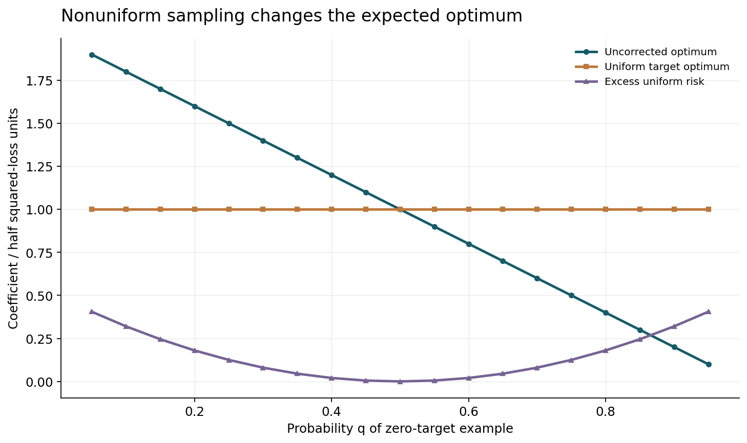
Let l_1(theta)=one half of(theta-0) squared and l_2(theta)=one half of(theta-2) squared. The uniform objective has optimum theta=1. If example one is sampled with probability q and example two with probability 1-q, the expected uncorrected gradient is theta-2(1-q), whose zero lies at 2(1-q).
Thus q=0.9 shifts the expected optimum to 0.2. A training curve can appear to improve rapidly on frequently sampled easy examples while moving away from the intended uniform optimum. The first figure plots this shifted optimum against q, together with excess uniform risk, which equals one half of(theta-1) squared. This is a constructed objective comparison, not a claim that any particular curriculum uses these losses. It shows why final evaluation must retain a fixed target measure. Measuring success only on the evolving sampled distribution can reward the sampler for avoiding the examples it has not learned.
5. Importance correction restores one expectation
For positive q_i, the estimator grad l_i/(N q_i) has expectation equal to the uniform average gradient over N examples. In the two-example model, the correction factors are 1/(2q) and 1/[2(1-q)]. The expected gradient is therefore theta-1 regardless of q, as long as both probabilities are positive.
This is a one-step conditional expectation statement. It does not establish equal trajectories, equal variance, or equal final performance under finite training. When q is close to zero or one, one correction factor becomes large and can increase variability. Clipping the correction weights changes the expectation again, generally introducing bias. A method may accept that tradeoff, but it should report it. The support condition matters too: if an example has zero sampling probability, no finite correction can recover its omitted contribution. A curriculum that temporarily excludes examples is therefore not simply an unbiased importance sampler for the full dataset during that phase.
6. Variance depends on the actual gradients
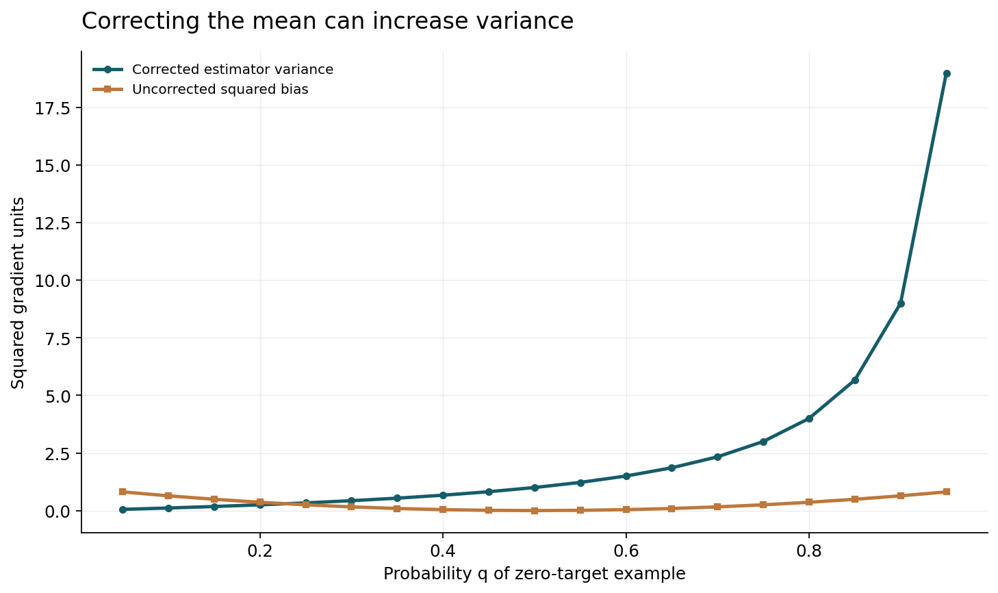
At theta=0 in our two-example problem, the uniform target gradient is negative one. The corrected estimator is zero when the first example is selected and -1/(1-q) when the second is selected. Its variance is q/(1-q), which grows without bound as q approaches one. Preferentially sampling the zero-gradient example is a poor variance-reduction policy at this point.
At another theta, the gradient magnitudes differ and so can the favorable sampling distribution. This explains why a difficulty score is not automatically an importance-sampling score. Loss magnitude, gradient norm, and expected future learning value are related only under additional assumptions. The second figure reports the exact corrected-gradient variance across q at the fixed stated theta, alongside the uncorrected bias. It illustrates a bias-variance tradeoff without claiming an optimal sampler for a neural network. A real adaptive sampler must pay for estimating useful scores and test whether their computational cost is repaid by better training progress.
7. Order can matter without changing total exposure
Even when both examples are used exactly once, sequential gradient updates depend on order. Starting from theta=0 with step size eta, processing the zero-target example then the two-target example gives theta=2eta. Reversing the order gives theta=2eta(1-eta). Their difference is 2eta squared.
Both sequences have identical example counts and the same nominal epoch. The discrepancy comes from evaluating the second gradient at a different parameter, not from unequal exposure. In more complex models, momentum, adaptive statistics, and nonlinear representations add further path dependence. This is why matching dataset size and number of epochs does not isolate a curriculum's mechanism. A useful experiment includes shuffled-order controls with exactly matched exposure and optimizer state conventions. The scalar identity provides a small falsification check: a simulator that reports identical endpoints for these two sequential schedules has likely averaged gradients or altered the update rule without acknowledging it.
8. A changing schedule need not imply a fixed objective
If q_t changes with time, the expected uncorrected update follows a sequence of weighted objectives. The final result depends on schedule duration, learning rates, and the point at which training stops. Even if the final phase uses the full target distribution, earlier phases can influence the initialization of that phase.
For a convex problem trained to its unique optimum under a sufficiently long final phase, some early differences may vanish. With finite budgets or nonconvex models, they may persist. Neither outcome can be assumed from the word curriculum. Report schedule time in actual updates or tokens, not only epochs when the sampled dataset size changes. A model-selected stopping rule may also favor one schedule through different validation exposure. Distinguishing a transient optimization aid from a persistent target change requires carefully matched terminal training and evaluation. The construction here isolates these possibilities without claiming which dominates in a particular deep architecture.
9. Difficulty is relative to a learner and a task
An example can be easy for one representation and difficult for another. A low current loss may indicate a well-learned pattern, a dominant class, an accidental shortcut, or an erroneous but easily memorized label. A high loss can indicate useful novelty, ambiguity, or corruption. Sorting by loss does not identify these causes.
An external teacher score supplies another information source with its own bias and cost. If the teacher has seen evaluation data, the curriculum can leak information into training even when the student has not. A defensible study documents the teacher's training scope and checks whether the score correlates with source, class, or annotation quality. It should also compare score direction: easy-first, hard-first, and matched random policies can reveal whether a proposed explanation is specific. A curriculum is most scientifically informative when its difficulty definition predicts testable differences rather than serving as a retrospective label for whichever order worked.
10. Selection can amplify blind spots
Self-paced selection may favor examples the current model already handles well. If a rare but valid category initially has high loss, it may be delayed or excluded, preventing the model from acquiring the features needed to learn it. That feedback loop can look like successful optimization on the selected subset.
Measure acceptance probabilities and cumulative exposure by category, source, and difficulty stratum where those attributes are available and appropriate. Include clean difficult examples and noisy easy examples as diagnostic controls. A policy with a positive exploration floor can prevent permanent exclusion, but the floor changes both computational efficiency and the induced objective. Its value must be tested rather than treated as a universal fix. The two-example model demonstrates the mathematical support issue in a minimal form: setting q=1 prevents any learning signal from the second example. Real data contain more nuanced versions of the same selection problem.
11. Prioritized replay has additional dependence
Experience replay samples from a buffer whose contents were produced by a behavior policy. Changing replay probabilities is only one part of the distribution shift. The environment, policy, temporal correlations, and buffer eviction rules determine which transitions are available at all.
Importance correction for replay frequency does not automatically correct every off-policy or bootstrapping bias. A reinforcement-learning study should state the target update being estimated and the approximation introduced by truncated weights, stale priorities, and target networks. Scores based on temporal-difference error can prioritize surprising transitions, but surprise may reflect noise rather than useful learning. Compare methods with matched interaction budgets as well as training compute, and include buffer-maintenance overhead. This review's independent finite dataset model deliberately omits those dependencies. It provides an accounting principle, not a complete theory of prioritized reinforcement learning or a guarantee of improved control performance.
12. Scoring overhead can erase apparent efficiency
A curriculum may require a teacher pass, per-example loss refreshes, gradient-norm estimates, sorting, or a distributed priority service. Reporting only student update time can make the method appear faster while moving computation outside the measured interval. Similarly, fewer updates need not mean fewer floating-point operations or less wall time.
A fair comparison includes preprocessing, score refresh frequency, data transfer, memory, and synchronization. If scores are reused from an earlier model, report that amortization assumption and the cost of obtaining the earlier model. Throughput should be measured under a consistent hardware and batch configuration. Statistical efficiency and systems efficiency are distinct: a method may reach a target loss in fewer examples yet take longer because selection is expensive. Both outcomes are useful if reported honestly. The exact arithmetic examples here have negligible scoring cost, so they cannot support any practical speedup claim. They isolate the statistical mechanism that a later systems experiment would need to evaluate.
13. Sampling and weighting need implementation tests
The intended probabilities should be checked against empirical draw frequencies on a synthetic dataset, including minimum-probability and zero-priority cases. Weight normalization should be tested separately from probability normalization. A common error is using minibatch-normalized importance weights while claiming an exact expectation that assumes a different estimator.
Distributed workers can use stale or inconsistent probabilities, and without recording the probability associated with each draw, the corresponding correction may be wrong. Replacement versus without-replacement sampling also changes the appropriate inclusion probabilities and variance formulas. The implementation contract should specify these details, not only the high-level scoring rule. Small exact cases are valuable because the correct expectation can be enumerated. They can detect a bias that a large noisy training curve would not reveal. A scientific result should bind its theoretical estimator to the actual sampler and weighting code used in the experiment.
14. An evaluation that distinguishes mechanisms
Freeze architecture, data splits, target risk, optimizer, and validation policy. Compare uniform sampling, uncorrected curriculum sampling, and corrected importance sampling. Add a shuffled exposure-matched schedule to separate order from frequency. Where a teacher supplies difficulty, include its cost and data scope.
Report cumulative per-example or per-stratum exposure, target evaluation loss, gradient-estimator diagnostics on controlled cases, and wall-clock resources. Evaluate both a fixed compute budget and time to a predeclared target metric. Include rare valid and noisy easy strata to test selection bias. For adaptive policies, retain score histories and probability versions so the actual training measure can be reconstructed. A result should explain whether the gain comes from reduced variance, a helpful temporary objective, representation path dependence, or changed population weighting. These explanations can coexist, but they should not be conflated.
15. What the finite program verifies
The program enumerates sampling outcomes for the two-example problem over a grid of q values. It checks the uncorrected expected optimum, exact importance-corrected expectation, and corrected variance at theta=0. Direct loss evaluation verifies the excess uniform risk shown in the first figure.
It also applies both sequential update orders over several step sizes and verifies their difference against 2eta squared. Boundary tests confirm that zero-probability support cannot use a finite importance correction and that uniform probabilities recover the ordinary estimator. The checks use no external packages or random neural training. They establish only the declared algebra and finite enumeration. Their role is to make claims about curriculum mechanisms precise enough to fail when an implementation or interpretation is wrong. They do not identify a universally useful difficulty metric or guarantee faster training on any particular benchmark.
16. Toward clearer claims about learning schedules
A curriculum is a policy over examples, time, and weights. Its scientific value depends on the target it is intended to optimize and the constraints it introduces along the path. Treating all nonuniform exposure as better teaching hides important changes in the statistical problem.
Open questions include predicting useful scores without costly oracle information, preserving rare-category exploration, and comparing adaptive policies under realistic systems budgets. Another challenge is understanding when early path differences survive a later common training phase. The finite constructions do not settle those questions, but they show why exposure, order, and importance correction must be recorded separately. A strong report states which mechanism is claimed, includes controls that could refute it, and measures the complete cost. That makes a curriculum result more useful than a metaphor about easy and hard lessons alone.
A completed epoch may not mean completed coverage.
With sampling with replacement, drawing N examples from a dataset of N items does not mean that every item was observed once. Under nonuniform probabilities, some examples may remain unseen for many nominal epochs. The probability that item i has not been sampled after T independent draws is (1-q_i)^T. This is an exposure statistic that can be computed exactly when probabilities are fixed.
For an easy-first policy with very small probability on difficult examples, the nominal update budget may therefore conceal a long delay before those examples contribute at all. A positive probability prevents permanent exclusion in an infinite sequence, but does not guarantee adequate finite-budget coverage. Reporting only expected counts Tq_i can also hide variability. A practical training audit can include the distribution of first-visit times, maximum gaps, and cumulative exposure by predefined strata.
Adaptive sampling complicates the formula because probabilities depend on training history. The actual policy log can still record when each example or stratum was eligible and what probability it received. This makes it possible to distinguish a failure to learn from a failure to present the information. The distinction matters for rare examples and for curricula that terminate before the full-data phase has run long enough.
The finite program checks the fixed-probability unseen-event formula against explicit enumeration for small budgets and verifies its monotonicity in q. These calculations complement the gradient-bias and order examples. They show that a curriculum experiment needs three accounting layers: the target objective, the update path, and the realized coverage. A favorable result on one layer does not establish adequacy on the others, particularly when training budgets are limited.
Core equations and definitions
(1) Uncorrected sampling generally changes the objective.
(2) Positive sampling probabilities and correct per-draw weights.
(3) Constructed targets zero and two, uniform target risk.
(4) Corrected estimator at theta=0 for the two-example model.
(5) Two sequential scalar SGD steps, initial theta zero.
Constructed analytical figures
Comparison and reporting contract
| Choice | What changes | What must be checked |
|---|---|---|
| Uncorrected sampling | Expected objective | Exposure and target weights |
| Importance correction | Mean preserved | Variance and support |
| Ordering only | Optimization path | Matched counts and optimizer state |
Evaluation protocol
- Fix target risk and validation policy.
- Compare corrected and uncorrected policies.
- Include shuffled exposure-matched controls.
- Account for scoring and teacher costs.
Limitations
- Finite quadratics do not reproduce deep curricula.
- Replay dependencies are excluded from the model.
- Unbiased one-step expectation does not imply equal trajectories.
Open research questions
- Which scores help without costly oracle information?
- How can rare examples retain finite-budget coverage?
- When do early path differences survive common final training?
Evidence and its boundaries
- Ordered training schedules introduce examples through a progression.
- [1] — Only the inspected abstract scope is asserted; no reproduction of source results. Inspected: Primary publisher or author arXiv abstract and metadata inspected via web on 2026-10-28; no independent proof or benchmark replication.
- Example selection can interact with the learner's current state.
- [2] — Only the inspected abstract scope is asserted; no reproduction of source results. Inspected: Primary publisher or author arXiv abstract and metadata inspected via web on 2026-10-28; no independent proof or benchmark replication.
- Curriculum policies are studied in deep-network training.
- [3] — Only the inspected abstract scope is asserted; no reproduction of source results. Inspected: Primary publisher or author arXiv abstract and metadata inspected via web on 2026-10-28; no independent proof or benchmark replication.
- Replay frequency can prioritize selected transitions.
- [4] — Only the inspected abstract scope is asserted; no reproduction of source results. Inspected: Primary publisher or author arXiv abstract and metadata inspected via web on 2026-10-28; no independent proof or benchmark replication.
- Importance sampling trades scoring costs against gradient variance.
- [5] — Only the inspected abstract scope is asserted; no reproduction of source results. Inspected: Primary publisher or author arXiv abstract and metadata inspected via web on 2026-10-28; no independent proof or benchmark replication.
- Minibatch sampling requires an explicit probability and complexity analysis.
- [6] — Only the inspected abstract scope is asserted; no reproduction of source results. Inspected: Primary publisher or author arXiv abstract and metadata inspected via web on 2026-10-28; no independent proof or benchmark replication.
References
- Curriculum Learning
Yoshua Bengio, Jérôme Louradour, Ronan Collobert, Jason Weston. Proceedings of the 26th International Conference on Machine Learning (2009). https://ronan.collobert.com/pub/matos/2009_curriculum_icml.pdfSource scope
Primary publisher or author arXiv abstract and metadata inspected via web on 2026-10-28; no independent proof or benchmark replication.
- Self-Paced Learning for Latent Variable Models
M. Pawan Kumar, Benjamin Packer, Daphne Koller. Advances in Neural Information Processing Systems (2010). https://papers.nips.cc/paper/2010/hash/e57c6b956a6521b28495f2886ca0977a-Abstract.htmlSource scope
Primary publisher or author arXiv abstract and metadata inspected via web on 2026-10-28; no independent proof or benchmark replication.
- On The Power of Curriculum Learning in Training Deep Networks
Guy Hacohen, Daphna Weinshall. Proceedings of the 36th International Conference on Machine Learning (2019). https://proceedings.mlr.press/v97/hacohen19a.htmlSource scope
Primary publisher or author arXiv abstract and metadata inspected via web on 2026-10-28; no independent proof or benchmark replication.
- Prioritized Experience Replay
Tom Schaul, John Quan, Ioannis Antonoglou, David Silver. arXiv preprint (2015). https://arxiv.org/abs/1511.05952Source scope
Primary publisher or author arXiv abstract and metadata inspected via web on 2026-10-28; no independent proof or benchmark replication.
- Not All Samples Are Created Equal: Deep Learning with Importance Sampling
Angelos Katharopoulos, François Fleuret. Proceedings of the 35th International Conference on Machine Learning (2018). https://proceedings.mlr.press/v80/katharopoulos18a.htmlSource scope
Primary publisher or author arXiv abstract and metadata inspected via web on 2026-10-28; no independent proof or benchmark replication.
- Importance Sampling for Minibatches
Dominik Csiba, Peter Richtárik. Journal of Machine Learning Research (2018). https://www.jmlr.org/papers/v19/16-241.htmlSource scope
Primary publisher or author arXiv abstract and metadata inspected via web on 2026-10-28; no independent proof or benchmark replication.