
Scientific Deep Learning / DEEP LEARNING III
Physics-Informed Learning Has a Scale: Residual Weighting, Units, and Error
Why residual units, boundary conditions and inverse stability determine what a physics-informed loss means.
English original. Translations of this new review are not yet available.

Abstract
Physics-informed models minimize residual objectives whose numerical scale and physical interpretation depend on units, sampling and boundary constraints. This analytical review separates objective equivalence from optimization stability and residual error from solution error. A scalar inconsistent-penalty construction gives an exact optimum and weight transformation under residual rescaling. A Dirichlet Poisson eigenmode construction shows frequency-dependent residual-to-field and residual-to-gradient relationships. Independent finite checks verify the identities, stability controls and an affine boundary counterexample. Six primary author records place these calculations alongside research on gradient imbalance, limiting-kernel behavior, failure modes, temporal ordering and domain decomposition. No neural network is newly trained, no source benchmark is reproduced, and no physical accuracy claim follows from the figures. A proposed evaluation protocol makes the units, norms, collocation measure and quantity of interest explicit.
In this paper
- 1. A small residual has no universal scale
- 2. What the selected primary records establish
- 3. Units enter the objective before optimization
- 4. A penalty compromise can be solved exactly
- 5. Invariance requires transforming the weight
- 6. Curvature changes with the residual scale
- 7. Residual error must pass through an inverse operator
- 8. Boundary error lives in a different component
- 9. Collocation is a sampling procedure
- 10. Local balance can hide a global failure
- 11. Evolutionary problems require a time contract
- 12. A proposed evaluation separates four error sources
- 13. What the executable controls do and do not test
- 14. A quantity of interest can demand another norm
- 15. From loss minimization to an auditable scientific claim
1. A small residual has no universal scale
Physics-informed learning invites a compelling inference: if a differentiable model nearly satisfies a differential equation, it should nearly solve the physical problem. The missing phrase is "in a specified norm, for a specified problem, with controlled boundary error." A residual is an output of an operator acting on an approximation. Its numerical magnitude depends on units, normalization, observation locations, and the operator's inverse. None of these disappears when the approximation is a neural network.
This review develops that distinction through two completely declared constructions. A quadratic penalty shows how changing the units of a residual changes the fitted compromise unless its weight changes accordingly. A one-dimensional Poisson example shows how residual frequency changes the relationship between residual norm and solution error. Both calculations can be reproduced without a neural training framework. They establish logical controls for evaluating physics-informed methods, not estimates of their accuracy on industrial simulations. The practical claim is modest but demanding: residual plots should be accompanied by dimensional conventions, separate component errors, and an independently evaluated quantity of interest.
2. What the selected primary records establish
Raissi, Perdikaris, and Karniadakis describe neural solution models constrained by differential equations. Wang, Teng, and Perdikaris investigate unbalanced back-propagated gradients in composite physics-informed losses. Wang, Yu, and Perdikaris analyze different loss-component convergence rates in a limiting neural-tangent-kernel regime. Krishnapriyan and colleagues demonstrate difficult optimization in selected convection, reaction, and diffusion settings. These are related observations, but they do not establish one universal diagnosis for every failed scientific neural model.
Two further directions change the organization of the task. Wang, Sankaran, and Perdikaris study temporal ordering in evolutionary problems, while Shukla, Jagtap, and Karniadakis investigate space and space-time domain decomposition. This review uses their publicly inspected author abstracts to identify those research directions. It does not independently verify their proofs, rerun their benchmarks, or transfer reported speed or accuracy factors to our constructions. The analysis below instead asks which measurements would distinguish a units problem, an optimization problem, an underresolved residual, and an unstable inverse problem. That distinction is necessary before deciding whether any proposed training modification addresses the actual cause.
3. Units enter the objective before optimization
Consider a field u with physical units U, a coordinate x with units L, and a second derivative u_xx with units U/L squared. Squaring a boundary mismatch and a PDE residual produces quantities with different units. Adding their bare numbers with a dimensionless coefficient silently chooses a conversion convention. Expressing length in millimeters rather than meters changes derivative magnitudes even when the physical field is unchanged. A loss value cannot be compared across those representations without tracking the transformation.
Nondimensionalization provides a principled place to declare this choice. Set x=L0 times xi and u=U0 times v. Derivatives and coefficients must then be transformed together; rescaling only the network input is insufficient. The resulting dimensionless groups describe the selected physical regime and remain in the equation. There is no universal scale that makes every problem equally well conditioned. However, a consistent transformation makes it possible to distinguish physical parameter changes from numerical changes in the training objective. A reproducibility record should retain L0, U0, residual normalization, boundary normalization, and the exact coefficient convention.
4. A penalty compromise can be solved exactly
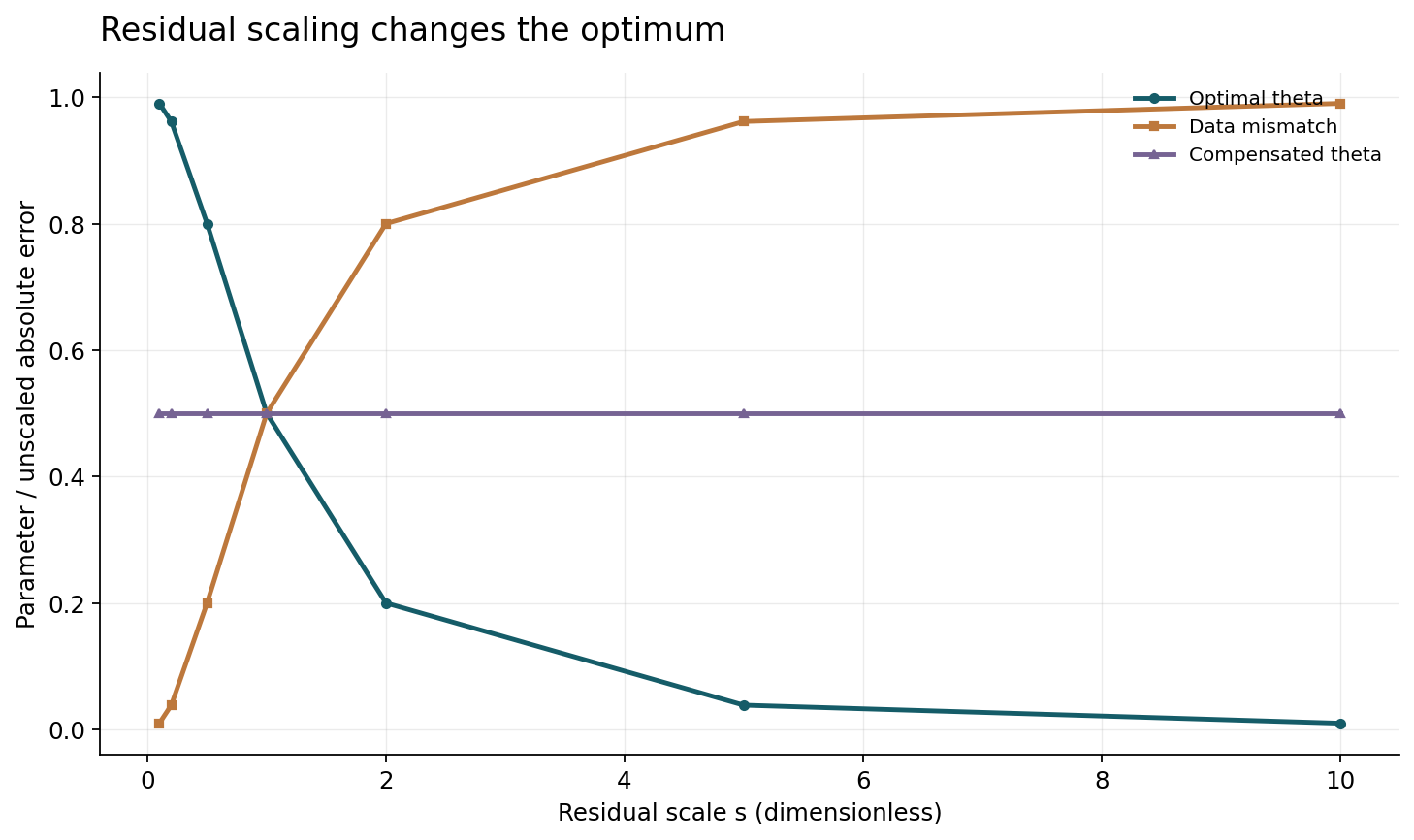
Let a scalar parameter theta face two inconsistent targets: a data term prefers theta=1 and a residual term prefers theta=0. Define L(theta)=(theta-1) squared plus lambda times (s theta) squared, with lambda positive and s a residual-unit scale. Differentiating gives theta_star=1/(1+lambda s squared). This is a deliberately elementary model of a soft-constraint compromise, not a discretization of a particular PDE. Its inconsistency is useful because an exactly satisfiable problem could hide weighting effects at the global zero-loss solution.
With lambda=1, s=0.1 gives theta_star approximately 0.990099, whereas s=10 gives approximately 0.009901. The underlying two desired targets did not change. Only the numerical scale of one penalty did. Figure 1 plots the fitted parameter and both unscaled errors over positive s. This example isolates a modeling choice that exists before questions of optimizer convergence or expressivity. Perfect minimization of an ambiguously scaled objective does not resolve that ambiguity. Conversely, a different optimum after unit conversion need not imply numerical instability; it may simply be the mathematically correct optimum of a different objective.
5. Invariance requires transforming the weight
If the residual is multiplied by s, choosing lambda_new=lambda_old/s squared preserves its contribution to the loss. In the scalar construction the optimum then remains exactly one half when the original lambda is one. The accompanying executable compares this analytic optimum with the zero of the derivative across multiple scales, and checks that the compensated objective agrees with the original at several trial parameters. These checks concern objective equivalence, not merely visually similar fitted curves.
This distinction helps evaluate adaptive weighting. A method that automatically balances gradient norms may produce useful optimization dynamics, but that is not the same guarantee as physical unit invariance. The gradients also depend on parameterization, current residual values, and which parameters are shared across components. Two physically equivalent coordinate systems can yield different parameter gradients. A convincing study should first demonstrate the intended transformation law on a controlled problem and then evaluate whether the adaptive rule respects it. Otherwise an apparent improvement may partly reflect a fortunate change in the effective relative penalties rather than a generally better solver.
6. Curvature changes with the residual scale
The scalar loss has curvature 2(1+lambda s squared). Gradient descent with step eta converges for this strictly convex quadratic when the absolute value of 1-2 eta(1+lambda s squared) is less than one. Thus a fixed learning rate can be stable at one residual scale and unstable at another even though both problems are easy to minimize in closed form. The construction separates changes in the optimum from changes in the iteration's stability: compensating the weight preserves both here, while adjusting only eta preserves neither the objective nor its optimum.
A multidimensional neural objective adds coupled directions, nonconvexity, and potentially very unequal curvature. The one-dimensional calculation cannot predict its entire spectrum. It does demonstrate why learning-rate sweeps should be conducted after the loss convention is frozen. Reporting only a successful final run obscures whether a method required extensive scale-dependent tuning. Useful reporting includes the original component losses, their gradients under a stated parameter metric, failed step sizes, stopping rules, and the computational budget used to select them. A solver comparison should not let one method hide more tuning in preprocessing.
7. Residual error must pass through an inverse operator
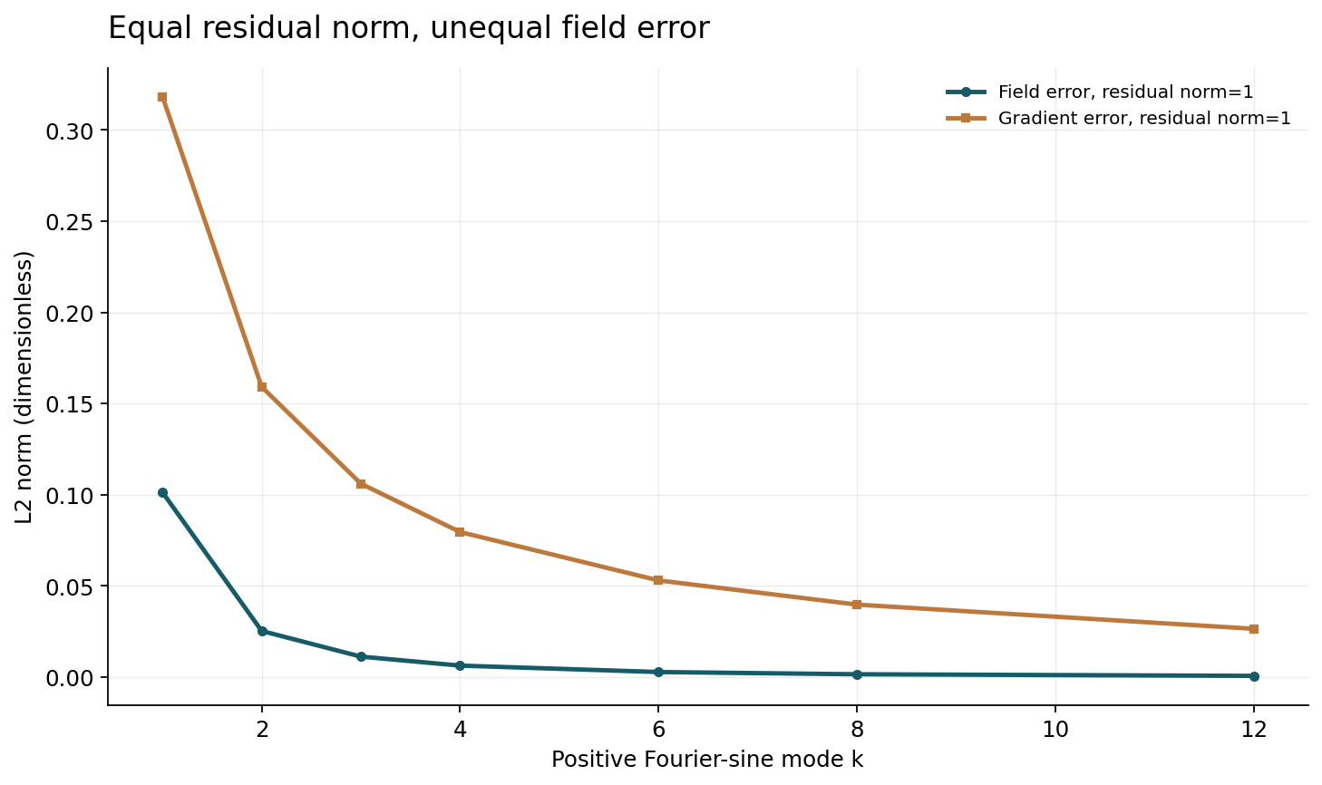
For the Dirichlet problem -u''=f on [0,1], let the approximation error e vanish at both endpoints. Its residual difference is r=-e''. If e(x)=a sin(k pi x), then r(x)=(k pi) squared a sin(k pi x). The L2 norms therefore satisfy norm(e)=norm(r)/(k pi) squared. The same residual norm can correspond to different solution errors at different frequencies. Figure 2 fixes the residual norm at one and plots the resulting solution error for positive integer modes.
This is an exact calculation for a linear, coercive, one-dimensional boundary-value problem with exact boundary conditions. It is not a universal residual-to-error theorem for nonlinear dynamics. Its purpose is to make the inverse-operator dependence visible. In a problem with poorly controlled boundary values, near-singular coefficients, nonunique solutions, or long-time instability, the relevant stability estimate may be weaker or require additional norms. A paper that reports only a small PDE residual leaves the reader unable to infer the field error unless those assumptions and constants are supplied or the field error is independently measured.
8. Boundary error lives in a different component
The Poisson mode calculation deliberately imposes zero error at both boundaries. Removing that condition reveals an immediate counterexample: e(x)=a+bx has zero second derivative for any a and b. A residual-only objective cannot distinguish these affine errors. Boundary measurements eliminate the ambiguity only if they actually constrain the relevant degrees of freedom. A finite penalty on noisy boundary values creates another compromise whose sensitivity should be analyzed separately.
Hard boundary parameterizations can help by constructing a trial function that satisfies a given condition exactly. They also change the approximation space and its derivatives. Multiplying a free network by x(1-x), for example, enforces homogeneous endpoints but may affect conditioning and the representation of boundary layers. The right comparison includes the entire parameterization, not merely the name of the network architecture. When boundary conditions are uncertain, exact enforcement can itself be inappropriate. The researcher should state whether the uncertainty belongs to the observations, the governing model, or the intended boundary-value problem rather than absorbing all discrepancies into a single training loss.
9. Collocation is a sampling procedure
A residual evaluated at a finite set of collocation points is an empirical quantity. It need not control residuals between those points. For a simple illustration, a smooth oscillation can vanish at a regularly spaced grid while being large between samples. Differentiation does not remove this possibility. Increasing network capacity without strengthening the validation design can therefore improve the sampled objective while leaving the continuous field poorly constrained.
Independent validation points should be selected before inspecting the trained residual landscape, or the selection procedure should be explicitly modeled. Adaptive collocation can deliberately concentrate training on difficult regions, but the resulting average no longer estimates a uniform-domain integral without appropriate weights. Both versions can be useful: one emphasizes worst regions, another estimates a physical integral. They answer different questions. Record the sampling measure, whether points are reused, the quadrature weights, and the distinction between training and validation coordinates. Reporting the total number of residual evaluations alone does not describe the information contained in those evaluations or the spatial coverage they achieve.
10. Local balance can hide a global failure
Partitioning a spatial or temporal domain creates local objectives and communication conditions. A small loss in every subdomain does not by itself guarantee a consistent global solution. Interfaces may require continuity of the field, flux, or another physically relevant trace. If these conditions are merely penalized, their scales and weights again become part of the model. A discontinuity can be concentrated on a thin interface and remain nearly invisible to an average interior residual.
An evaluation should include explicit interface checks and a global quantity of interest. For conservation laws, this might involve comparing fluxes across an interface and measuring a domain-wide balance, with the discretization error of that measurement stated. Time decomposition likewise requires accurate propagation of the state that initializes the next interval. Error accumulated in an early interval cannot be wished away by small later local training losses. These are analytical obligations created by the decomposition itself. They do not contradict the potential computational advantages of local training; they specify what must be checked before those advantages become scientifically interpretable.
11. Evolutionary problems require a time contract
For a time-dependent system, a surrogate may represent the whole space-time field at once or repeatedly predict the next state. These are different approximation procedures with different error propagation. A global space-time objective can trade errors in early and late regions according to its weighting. An autoregressive procedure can accumulate local errors through repeated use of its own predictions. A model chosen for low average space-time residual might therefore fail a forecast requirement focused on an early transient or a late instability.
State clearly whether the task is interpolation of a known trajectory, conditional solution of an initial-value problem, or forecasting beyond observed time. Initial conditions, forcing availability, and test horizons must match the intended use. A causal training schedule changes optimization order; it does not establish that unknown future forcing has become available. Long-horizon evaluation should measure trajectories and physical invariants under unseen initial conditions, with uncertainty and failure cases retained. The word causal has a numerical ordering meaning in this context that should not be confused with identifying causal effects from observational data.
12. A proposed evaluation separates four error sources
A practical study can begin with manufactured solutions whose exact derivatives and forcing are known. First fix the physical problem and its nondimensional form. Next vary residual scaling while applying the analytically required weight transformation. Then vary collocation density and sampling strategy while evaluating on an independent dense grid or trustworthy quadrature. Finally compare optimization budgets and stopping rules with the model class held fixed. This sequence helps separate objective changes from approximation, sampling, and optimization error.
The study should report boundary, interior, interface, and quantity-of-interest errors independently. When a reference numerical solver is used, its own convergence and tolerance need documentation. Comparing a neural approximation with one coarse numerical solution does not establish continuum accuracy. Training cost, residual evaluation cost, and amortized inference cost should also be separated; repeated prediction over many parameter instances is different from solving one instance. These proposed controls are not newly executed neural experiments in this review. They are a concrete specification for evidence that would justify stronger statements than those supported by the finite constructions included here.
13. What the executable controls do and do not test
The public standard-library program evaluates the scalar optimum, compensated weights, derivative zeros, quadratic stability factors, and the Poisson eigenmode relation. It also checks an affine boundary-error counterexample and compares analytic integrals with a numerical quadrature on representative modes. Figure data are generated from those same declared functions, so a reader can inspect every parameter and recompute every point without external datasets or model weights.
This transparency should not be mistaken for physical validation. The program has no fluid solver, no learned architecture, and no real material measurements. Its strongest conclusions are conditional identities and counterexamples. It cannot rank PINN implementations, establish the accuracy of cited algorithms, or provide uncertainty intervals for an engineering decision. A useful finite model is valuable precisely because it makes the scope narrow enough to verify. The corresponding research challenge is to determine which of its mechanisms remain dominant when many scales, uncertain boundaries, nonlinear dynamics, and finite optimization interact. That challenge requires new experiments beyond the calculations offered here.
14. A quantity of interest can demand another norm
Suppose the desired output is the value at a particular point rather than the field's average squared error. A small L2 field error need not control that pointwise value without additional regularity. Likewise, a flux depends on a derivative, so an approximation can have a small field error and a relatively large flux error. The evaluation norm should be chosen to support the actual scientific question. It is not enough to report whichever norm is most convenient for the training code.
In the Poisson mode construction, the derivative error has amplitude k pi times the field-error amplitude. Fixing field error while increasing frequency increases derivative error. Fixing residual error instead decreases field and derivative errors at different rates. These elementary relationships explain why apparently inconsistent rankings can arise when studies compare different outputs. A solver optimized for a field norm can be unsuitable for a boundary flux without being mathematically defective. The research claim should name both the target functional and the validation method used to estimate it.
A further complication is inverse identification of physical coefficients. A small forward residual can coexist with poorly identified parameters when multiple coefficient-field combinations explain the observations. Adding residual points does not necessarily add independent information about the coefficient. A proposed inverse-problem study should vary the measurement locations and forcing conditions, report parameter sensitivity, and distinguish uncertainty in the field from uncertainty in the governing coefficient. The finite checks here do not solve that inverse problem; they show why a forward residual alone cannot serve as its complete validation.
15. From loss minimization to an auditable scientific claim
A strong physics-informed result connects a chain of statements: the intended physical problem, its representation in chosen units, the numerical objective, the optimization procedure, the measured errors, and the deployment quantity of interest. Each link can fail while the others look persuasive. A smooth plotted solution and a rapidly falling loss curve do not repair a missing link. Neither does a large architecture or a claim of using the governing equation.
The two constructions suggest a compact reporting discipline. Show how the objective transforms under units, identify the norm in which residuals are evaluated, separate boundary constraints from interior physics, and test residual-to-solution implications rather than assuming them. Preserve collocation and optimizer choices as part of the executable specification. Future work can examine whether scale-aware objectives and certified independent residual evaluation produce more reliable selection among scientific neural models. Until then, the most defensible conclusion is conditional: learning physics through residuals can be useful, but a residual acquires scientific meaning only after its scale, domain, sampling measure, and stability relationship have been made explicit.
Core equations and definitions
(1) Dimensionless scalar construction: the two soft targets conflict; s rescales only the residual number.
(2) Unique optimum for lambda>0; derivative and curvature are checked independently.
(3) This weight compensates multiplying a residual by s, preserving the original objective.
(4) Homogeneous Dirichlet Poisson mode on [0,1], k a positive integer.
(5) Exact L2 relation for this mode; not a general nonlinear PDE bound.
Constructed analytical figures
Comparison and reporting contract
| Diagnostic | What it establishes | What remains unproved |
|---|---|---|
| Loss value | Objective under declared normalization | Physical solution accuracy |
| Boundary check | Selected boundary mismatch | Interior solution correctness |
| Independent residual | Residual under validation measure | Unstated inverse stability |
| Quantity of interest | Accuracy of selected functional | All other scientific outputs |
Evaluation protocol
- Freeze nondimensional variables and transformed coefficients.
- Test residual scaling with compensating weights.
- Validate boundary and interface errors separately.
- Use independent residual points and explicit quadrature.
- Compare with a converged reference solver and report total training cost.
Limitations
- No neural training or physical measurements are performed.
- The scalar compromise is not a PDE solver.
- The eigenmode result requires homogeneous boundaries and a linear Poisson operator.
- Only primary abstracts and metadata were inspected; proofs are not independently audited.
Open research questions
- Can scale-aware objectives preserve performance under equivalent physical units?
- Which residual norms best control the intended functional?
- How can adaptive collocation retain interpretable validation measures?
Evidence and its boundaries
- PDE constraints are incorporated in neural solution models.
- [1] — Scope-level source statement only; no independent reproduction, priority ranking or theorem-proof audit. Inspected: Primary author abstract and bibliographic record.
- Composite residual losses can have unbalanced back-propagated gradients.
- [2] — Scope-level source statement only; no independent reproduction, priority ranking or theorem-proof audit. Inspected: Primary author abstract and bibliographic record.
- The studied limiting-kernel regime exposes unequal convergence of loss components.
- [3] — Scope-level source statement only; no independent reproduction, priority ranking or theorem-proof audit. Inspected: Primary author abstract and bibliographic record.
- Soft PDE regularization can cause difficult conditioning in studied examples.
- [4] — Scope-level source statement only; no independent reproduction, priority ranking or theorem-proof audit. Inspected: Primary author abstract and bibliographic record.
- Temporal loss organization is investigated for evolutionary PDE training.
- [5] — Scope-level source statement only; no independent reproduction, priority ranking or theorem-proof audit. Inspected: Primary author abstract and bibliographic record.
- Space and space-time subdomain methods allow local training choices.
- [6] — Scope-level source statement only; no independent reproduction, priority ranking or theorem-proof audit. Inspected: Primary author abstract and bibliographic record.
References
- Physics Informed Deep Learning (Part I): Data-driven Solutions of Nonlinear Partial Differential Equations
Maziar Raissi, Paris Perdikaris, George Em Karniadakis. arXiv author manuscript (2017). https://arxiv.org/abs/1711.10561Source scope
Primary author record title, complete author list, submission history and abstract inspected through web tools on 2026-10-28. Full proof and benchmark execution not independently checked.
- Understanding and mitigating gradient pathologies in physics-informed neural networks
Sifan Wang, Yujun Teng, Paris Perdikaris. arXiv author manuscript (2020). https://arxiv.org/abs/2001.04536Source scope
Primary author record title, complete author list, submission history and abstract inspected through web tools on 2026-10-28. Full proof and benchmark execution not independently checked.
- When and why PINNs fail to train: A neural tangent kernel perspective
Sifan Wang, Xinling Yu, Paris Perdikaris. arXiv author manuscript (2020). https://arxiv.org/abs/2007.14527Source scope
Primary author record title, complete author list, submission history and abstract inspected through web tools on 2026-10-28. Full proof and benchmark execution not independently checked.
- Characterizing possible failure modes in physics-informed neural networks
Aditi S. Krishnapriyan, Amir Gholami, Shandian Zhe, Robert M. Kirby, Michael W. Mahoney. arXiv author manuscript (2021). https://arxiv.org/abs/2109.01050Source scope
Primary author record title, complete author list, submission history and abstract inspected through web tools on 2026-10-28. Full proof and benchmark execution not independently checked.
- Respecting causality is all you need for training physics-informed neural networks
Sifan Wang, Shyam Sankaran, Paris Perdikaris. arXiv author manuscript (2022). https://arxiv.org/abs/2203.07404Source scope
Primary author record title, complete author list, submission history and abstract inspected through web tools on 2026-10-28. Full proof and benchmark execution not independently checked.
- Parallel Physics-Informed Neural Networks via Domain Decomposition
Khemraj Shukla, Ameya D. Jagtap, George Em Karniadakis. arXiv author manuscript (2021). https://arxiv.org/abs/2104.10013Source scope
Primary author record title, complete author list, submission history and abstract inspected through web tools on 2026-10-28. Full proof and benchmark execution not independently checked.