
Scientific Deep Learning / DEEP LEARNING III
Learning an Operator Across Grids: Resolution, Aliasing, and What Transfers
Parameter sharing across grids is weaker than recovering information removed by sampling.
English original. Translations of this new review are not yet available.

Abstract
This review analyzes resolution transfer as a composition of sampling, array computation and reconstruction. Two periodic functions that alias on a coarse grid produce distinct inverse-Laplacian outputs, yielding a triangle-inequality lower bound for any predictor that receives only the shared samples. A separate finite Fourier construction decomposes truncation and multiplier-estimation errors. The reproducible figures illustrate input-information limits and an error floor that larger retained bandwidth does not remove. Six primary records cover Fourier operators, function-space formulations, DeepONet, error decompositions, representation equivalence and convolutional operators. Their scope is reviewed without reproducing neural benchmarks. The proposed evaluation distinguishes input from output resolution, nonlinear aliasing, quadrature, boundary conventions and target-solver error.
In this paper
- 1. An array is a representation of a function
- 2. What the primary literature contributes
- 3. The task needs three maps, not one
- 4. Coarse samples cannot distinguish aliases
- 5. A two-input lower bound follows directly
- 6. More output pixels do not create more observations
- 7. Truncation and coefficient error behave differently
- 8. Nonlinearity can create unresolved frequencies
- 9. Quadrature determines the discrete integral
- 10. Boundary conditions complicate spectral language
- 11. The target solver contributes another approximation
- 12. Cross-resolution experiments need independent axes
- 13. A proposed stress suite tests the representation contract
- 14. Conservation provides a separate diagnostic
- 15. Resolution transfer is conditional information transfer
1. An array is a representation of a function
A neural operator is often introduced as a model that maps one function to another. A computer receives arrays, however, and those arrays depend on sensors, grids, quadrature, interpolation, and boundary conventions. Reusing the same learned parameters on a larger array is a useful capability, but it does not alone prove that the implemented computation represents the same continuous operator. The distinction matters most when an input contains structure that the training grid could not observe.
This review studies resolution transfer through explicit sampling and approximation questions. A Fourier aliasing example constructs two continuous inputs that are identical on a coarse grid but produce different outputs under a chosen operator. A second example separates truncation error from parameter error in a diagonal Fourier map. Both are finite analytical controls, not newly trained neural-operator benchmarks. They expose why resolution, information, and accuracy should be reported separately. A model can accept arbitrary grid sizes while lacking the information or learned coefficients needed for accurate transfer. Conversely, a carefully restricted function class can make a coarse representation sufficient.
2. What the primary literature contributes
Li and colleagues introduce a Fourier-parameterized neural operator for families of PDE problems. Kovachki and colleagues formulate neural operators in function spaces and discuss parameter sharing across discretizations. The original DeepONet manuscript by Lu, Jin, and Karniadakis distinguishes sensor encoding from evaluation at output coordinates. Lanthaler, Mishra, and Karniadakis analyze encoding, approximation, and reconstruction errors. These records motivate the distinction between representation and the function being represented.
Bartolucci and colleagues explicitly examine operator aliasing and representation equivalence. Raonic and colleagues design convolutional neural operators to preserve a continuous interpretation under discretization. We use the inspected primary abstracts for these scope-level statements; theorem hypotheses and reported benchmark improvements are not independently reproduced here. The present constructions are our own calculations on periodic scalar functions. They are intentionally simpler than the nonlinear PDE maps studied in the papers. Their role is to identify counterexamples that a resolution-transfer claim should exclude, not to claim that any named architecture necessarily fails on its published test distribution.
3. The task needs three maps, not one
Let S_h sample an input function on a grid with spacing h, let F_h act on the resulting array, and let R_h reconstruct a continuous output. The implemented approximation is R_h F_h S_h. A claim about an underlying operator G should compare this composition with G on a declared class of input functions. Without specifying S_h and R_h, an error measured on arrays has no unique function-space interpretation.
The sampling map may be point evaluation, cell averaging, a sensor integral, or a projection onto basis coefficients. These are not interchangeable near discontinuities or for unresolved oscillations. Reconstruction can likewise introduce assumptions: piecewise constants, linear interpolation, and spectral interpolation behave differently. A discretization-independent parameter vector only addresses how F_h is represented. It says nothing by itself about whether S_h retains sufficient information or R_h preserves the target norm. An experimental report should identify all three maps and explain how they change across resolutions. Otherwise a favorable fine-grid result could mainly reflect a particular interpolation convention rather than a learned continuous relationship.
4. Coarse samples cannot distinguish aliases
On the periodic interval [0,1), sample x_j=j/N for j from zero to N-1. The complex modes exp(2 pi i k x) and exp(2 pi i (k+N)x) have identical samples because exp(2 pi i j)=1. For real cosine inputs, the same equality holds pointwise on the grid. No deterministic or randomized estimator receiving only this array can determine which of the two continuous inputs generated it without additional assumptions or information.
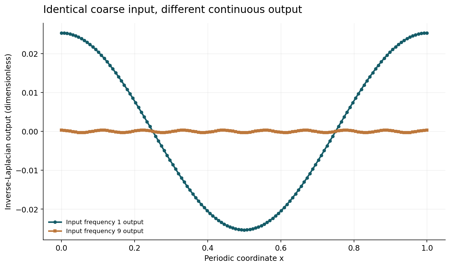
Choose an operator that multiplies Fourier mode k by m(k). If m(k) differs from m(k+N), the desired outputs differ even though the observed input arrays coincide. This creates an information limitation before training begins. The architecture can only resolve it by using a restricted prior, additional sensors, or another source of information. A successful prediction on a distribution containing only low-frequency inputs is consistent with this limitation. It does not establish recovery of arbitrary high-frequency structure. Figure 1 makes the ambiguity visible using a coarse grid of eight samples and cosine frequencies one and nine, then evaluates their operator outputs on a dense independent grid.
5. A two-input lower bound follows directly
Suppose two admissible functions a and b have identical sampled inputs and the corresponding target functions are G(a) and G(b). Any single reconstructed prediction p must serve both. By the triangle inequality, at least one of the two errors is at least half the distance between G(a) and G(b) in the chosen norm. This elementary lower bound does not depend on the size of the neural network, the optimizer, or the number of training examples.
For our construction, G is the periodic mean-zero inverse of minus the second derivative. Its multiplier is 1/(2 pi k) squared for nonzero k. The outputs of the one-cycle and nine-cycle cosine inputs therefore differ in amplitude and frequency. Their L2 separation can be computed exactly from orthogonality. The code verifies the indistinguishable input arrays and the output separation. The lower bound applies to a class containing both inputs under the same sampling operator. It does not apply unchanged when a sensor measures derivatives, an auxiliary label identifies frequency, or the admissible function class excludes the high-frequency input. Those are meaningful changes to the information available.
6. More output pixels do not create more observations
Evaluating an output on a denser grid can reduce reconstruction error for a function already represented by the model. It cannot, by itself, recover input distinctions removed by the sampling map. This is the central difference between output-coordinate flexibility and input-information sufficiency. A model may generate a smooth high-resolution field because its learned prior favors smoothness, even when the actual unresolved input would lead to another field.
The phrase super-resolution should therefore identify which side of the operator is refined. Are additional input measurements available, or only more output coordinates? Is the fine output compared against an independently converged solver, or against an interpolation of a coarse target? Is the test input sampled from the same smoothness class used in training? These questions define the inference problem. A dense visual rendering can be useful for downstream numerical integration, but visual detail is not evidence of newly recovered physical information. The model's uncertainty should reflect unresolved alternatives when the task permits multiple continuous inputs consistent with the same observations.
7. Truncation and coefficient error behave differently
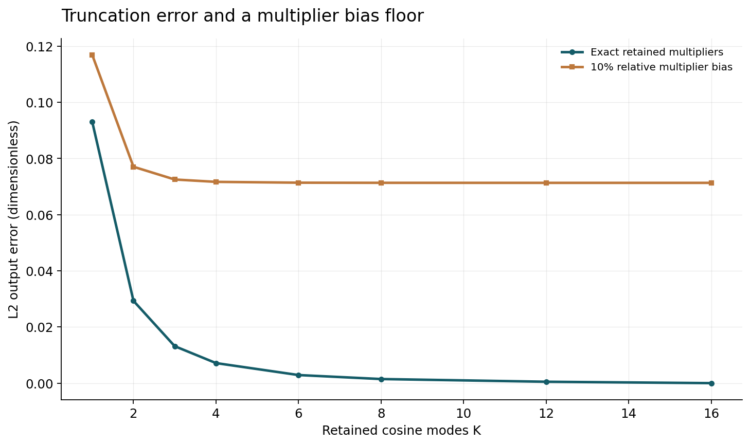
Consider a target operator diagonal in a Fourier basis, with known input coefficients a_k and multipliers m_k. A truncated approximation retains modes up to K and uses estimated multipliers mhat_k. By orthogonality, its squared L2 error separates into retained-mode coefficient error and omitted-mode target energy, using a consistent normalization of the real basis. Increasing K reduces the truncation part if the coefficients are accurate, but it can introduce additional estimation errors when newly included multipliers are poorly learned.
Figure 2 uses cosine coefficients a_k=1/k and a smoothing multiplier m_k=1/k squared over a finite set of modes. One curve uses exact retained multipliers, while another introduces a declared fixed relative error on retained modes. This is an analytical sensitivity study, not a measured learning curve. The exact curve approaches zero when all modeled modes are retained. The biased curve reaches a nonzero floor because representation capacity does not remove coefficient error. The construction helps interpret ablations in which mode count changes together with parameter count, optimization difficulty, and sample complexity. More retained frequencies are not an unqualified accuracy guarantee.
8. Nonlinearity can create unresolved frequencies
Even when an input is band-limited, applying a nonlinear pointwise transformation can create higher frequencies. Squaring cos(2 pi k x), for example, yields a constant term and a cosine at frequency 2k. If the computational grid cannot represent the doubled frequency, a discrete implementation can alias it into a lower one. Consequently, truncating the initial input does not automatically make every later nonlinear layer alias-free.
An implementation that claims a continuous interpretation should specify how it handles these newly created frequencies: oversampling, filtering, projection, or a restricted nonlinear representation. Each choice changes the effective operator. Filtering can prevent aliasing but discard information that the target task needs. Oversampling can increase memory and compute. The correct design depends on the declared function class and acceptable approximation error. A benchmark that evaluates only one resolution may not reveal the difference because train and test share the same aliasing convention. Cross-grid tests should therefore include controlled inputs near the representable-frequency boundary and compare against the intended continuous transformation.
9. Quadrature determines the discrete integral
Integral-kernel formulations require numerical integration when implemented on a grid or point cloud. Equal-weight sums approximate different measures depending on how points are distributed. On a nonuniform grid, using a simple average can overweight densely sampled regions. A model trained under that convention may learn to compensate on one sampling pattern and fail when the pattern changes, even if the physical input function is unchanged.
Quadrature weights should be treated as part of the sampling representation, not an incidental coding detail. For a constant function and an integral operator, the sum of weights provides a simple invariant to check. More demanding controls use polynomials or Fourier modes whose integrals are known. Tests should compare both coordinates and weights across discretizations. On irregular domains, geometric preprocessing and boundary handling also enter the computation. None of these observations implies that a learned operator must use classical quadrature exclusively. They imply that a learned aggregation rule needs its own evidence of consistency under the distribution of point sets where it will be used.
10. Boundary conditions complicate spectral language
Our aliasing construction is periodic. Many physical domains are not. Applying a periodic Fourier transform to nonperiodic data can create discontinuities at the artificial boundary, altering spectral decay and the difficulty of approximation. Padding, coordinate embeddings, boundary extensions, and domain mappings can reduce some practical difficulties, but they change the representation and should be documented.
Boundary conditions can also be inputs to the operator rather than fixed assumptions. Generalizing over forcing functions while holding boundaries fixed is a different task from generalizing over geometry or boundary type. A reported cross-resolution result on one domain should not be described as cross-geometry generalization without evidence. For an irregular domain, the physical distance represented by adjacent array indices may vary, so array convolution and physical locality diverge. Evaluation should include the intended boundary values, fluxes, and conservation properties alongside global field norms. Small average error can coexist with a boundary defect that dominates a downstream physical calculation.
11. The target solver contributes another approximation
Supervised operator learning often uses outputs generated by a numerical solver. The target is therefore initially a discrete solver map, which may approximate a continuous physical operator only under its own convergence assumptions. Learning that map accurately is worthwhile, but it does not establish accuracy beyond the target solver's discretization or model error. A finer neural output cannot be certified by comparing it only with interpolated coarse training targets.
A useful evaluation hierarchy includes a target-solver convergence study, held-out input functions, and at least one independent higher-accuracy reference on selected cases. The computational cost of generating training data belongs in an amortization analysis. Inference may be fast after training, while total cost is favorable only after enough queries or in a setting where training data already exist. Separating these costs prevents a misleading comparison between one neural forward pass and an entire classical solve. The number of queries, accuracy tolerance, hardware, and preprocessing must be matched. This review offers no measured speed comparison; the point is to define the accounting required for one.
12. Cross-resolution experiments need independent axes
Resolution transfer should be evaluated along several axes rather than compressed into one score. Input resolution, output resolution, coefficient bandwidth, physical parameters, geometry, and time horizon can all change independently. A model might transfer across output grids within the same bandwidth while failing when input measurements become coarser. It might handle the same PDE at new grids but fail when a parameter moves beyond the training range.
A practical matrix freezes all but one axis initially, then includes selected interactions. Start with analytically controlled periodic functions, add nonlinear operators, and finally evaluate the target PDE family. For each case record interpolation rules, quadrature weights, normalization, and whether fine-grid target data influenced selection. Include a reconstruction-only baseline that uses the coarse solver or input representation without a learned operator. This helps determine whether the reported gain comes from learned dynamics or simply from a strong interpolation prior. Repeated seeds address optimization variation, while multiple independent input functions address generalization; treating spatial grid points as independent replicates overstates the amount of evidence.
13. A proposed stress suite tests the representation contract
The executable accompanying this review checks exact coarse-grid aliasing, the two-input output separation, finite spectral error decomposition, and frequency creation under squaring. It includes low-frequency positive controls that are well resolved, high-frequency negative controls that alias, and the full-retention endpoint of the truncation calculation. Numerical quadrature is compared with analytic norms at increasing evaluation resolution, so the verification procedure itself has a visible convergence check.
A neural implementation could adopt these controls without treating them as a complete benchmark. The model should first reproduce basic invariances under consistent changes of grid representation. Then it should disclose where the controls fall outside its training distribution or function class. Failure on an excluded input is not necessarily a design defect; failing to state the exclusion is a scientific interpretation problem. Conversely, passing a handful of sinusoidal controls does not establish nonlinear PDE generalization. The stress suite is useful because its expected outcomes are explicit, allowing a researcher to locate errors in sampling, reconstruction, parameterization, or evaluation before investing in a larger empirical study.
14. Conservation provides a separate diagnostic
A low field error and a small conservation defect are different measurements. An approximation may preserve an integral exactly while distributing the field incorrectly, or match most point values while violating a balance important to long-time behavior. For a periodic problem, the zero Fourier mode often represents a domain average. A truncation rule that retains this mode can preserve that average even when higher modes are inaccurate. That success should not be generalized to arbitrary fluxes or nonlinear invariants.
Our inverse-Laplacian construction explicitly excludes the zero mode because the periodic operator has a constant nullspace. This restriction is part of the problem definition. Including a nonzero-mean forcing would require a different solvability treatment; silently setting its inverse multiplier to zero would change the task. A numerical implementation should test both admissible mean-zero inputs and rejected or separately handled inadmissible inputs. Such edge cases reveal whether mathematical assumptions survive the data pipeline.
For learned PDE maps, useful diagnostics can include mass balance, boundary flux, positivity, and monotonicity where those properties belong to the physical problem. They should be measured on independent cases and with a numerical procedure whose error is understood. Imposing one property architecturally may improve reliability, but it can also restrict the approximation class. The tradeoff should be evaluated at matched accuracy and computation rather than asserted from the presence of a constraint. Resolution transfer becomes more informative when it preserves the intended physical properties as well as an array-shaped output.
15. Resolution transfer is conditional information transfer
The strongest defensible claim links an admissible input class, a sampling rule, a learned map, and a reconstruction norm. Within that contract, shared parameters and continuous formulations can provide valuable flexibility. Outside it, increasing resolution can reveal a previously hidden error rather than improve the solution. That is not paradoxical: a finer grid can measure distinctions that the original experiment was unable to see.
Future work should report uncertainty over unresolved inputs, distinguish representation error from learned coefficient error, and test whether alias-control mechanisms remain effective through nonlinear layers. An especially useful result would quantify when additional sensors are more valuable than additional model capacity. Our constructions establish only finite mathematical examples, but they offer a clear standard for interpretation. A model that runs on many grids has demonstrated computational compatibility. A model that remains accurate on independently verified continuous tasks has demonstrated something stronger. The difference should be visible in the methods, figures, and claims rather than left for readers to infer from the phrase neural operator.
Core equations and definitions
(1) Sampling S_h, array map F_h and reconstruction R_h jointly define the implemented function-space approximation.
(2) Modes k and k+N alias at the N periodic grid points.
(3) If sampled a and b coincide, a single prediction faces this triangle-inequality lower bound.
(4) Multiplier of the periodic mean-zero inverse of minus the second derivative.
(5) Finite cosine expansion with orthogonal modes and L2 norm on [0,1]; real-cosine normalization supplies one half.
Constructed analytical figures
Comparison and reporting contract
| Diagnostic | What it establishes | What remains unproved |
|---|---|---|
| New output grid | Coordinate evaluation flexibility | Recovery of missing input frequencies |
| Shared weights | Parameter compatibility | Discrete-continuous equivalence |
| Low field error | Accuracy in selected norm | Conservation or derivative accuracy |
| Fast forward pass | Inference cost | Amortized end-to-end savings |
Evaluation protocol
- Specify sampling and reconstruction maps.
- Separate input and output resolution changes.
- Test alias pairs and nonlinear frequency generation.
- Document quadrature and zero-mode conventions.
- Use independent fine references and disclose solver convergence.
Limitations
- No learned operator is trained here.
- Examples are periodic scalar finite Fourier constructions.
- The lower bound assumes the admissible class includes both aliased inputs.
- Source proofs and numerical results are not independently reproduced.
Open research questions
- When are additional sensors more useful than more retained modes?
- How does nonlinear alias control trade accuracy against compute?
- Can uncertainty reflect the family of inputs consistent with coarse samples?
Evidence and its boundaries
- Fourier-parameterized kernels learn PDE solution maps.
- [1] — Scope-level source statement only; no independent reproduction, priority ranking or theorem-proof audit. Inspected: Primary author abstract and bibliographic record.
- Function-space operator parameterizations share parameters across discretizations.
- [2] — Scope-level source statement only; no independent reproduction, priority ranking or theorem-proof audit. Inspected: Primary author abstract and bibliographic record.
- Sensor encoding and output-coordinate decoding define an operator-learning architecture.
- [3] — Scope-level source statement only; no independent reproduction, priority ranking or theorem-proof audit. Inspected: Primary author abstract and bibliographic record.
- Encoding, approximation and reconstruction errors are separately analyzed.
- [4] — Scope-level source statement only; no independent reproduction, priority ranking or theorem-proof audit. Inspected: Primary author abstract and bibliographic record.
- Operator aliasing distinguishes continuous operators from discrete implementations.
- [5] — Scope-level source statement only; no independent reproduction, priority ranking or theorem-proof audit. Inspected: Primary author abstract and bibliographic record.
- Convolution-based operators are designed to preserve continuous structure.
- [6] — Scope-level source statement only; no independent reproduction, priority ranking or theorem-proof audit. Inspected: Primary author abstract and bibliographic record.
References
- Fourier Neural Operator for Parametric Partial Differential Equations
Zongyi Li, Nikola Kovachki, Kamyar Azizzadenesheli, Burigede Liu, Kaushik Bhattacharya, Andrew Stuart, Anima Anandkumar. arXiv author manuscript (2020). https://arxiv.org/abs/2010.08895Source scope
Primary author record title, complete author list, submission history and abstract inspected through web tools on 2026-10-28. Full proof and benchmark execution not independently checked.
- Neural Operator: Learning Maps Between Function Spaces
Nikola Kovachki, Zongyi Li, Burigede Liu, Kamyar Azizzadenesheli, Kaushik Bhattacharya, Andrew Stuart, Anima Anandkumar. arXiv author manuscript (2021). https://arxiv.org/abs/2108.08481Source scope
Primary author record title, complete author list, submission history and abstract inspected through web tools on 2026-10-28. Full proof and benchmark execution not independently checked.
- DeepONet: Learning nonlinear operators for identifying differential equations based on the universal approximation theorem of operators
Lu Lu, Pengzhan Jin, George Em Karniadakis. arXiv author manuscript (2019). https://arxiv.org/abs/1910.03193Source scope
Primary author record title, complete author list, submission history and abstract inspected through web tools on 2026-10-28. Full proof and benchmark execution not independently checked.
- Error estimates for DeepOnets: A deep learning framework in infinite dimensions
Samuel Lanthaler, Siddhartha Mishra, George Em Karniadakis. arXiv author manuscript (2021). https://arxiv.org/abs/2102.09618Source scope
Primary author record title, complete author list, submission history and abstract inspected through web tools on 2026-10-28. Full proof and benchmark execution not independently checked.
- Representation Equivalent Neural Operators: a Framework for Alias-free Operator Learning
Francesca Bartolucci, Emmanuel de Bézenac, Bogdan Raonić, Roberto Molinaro, Siddhartha Mishra, Rima Alaifari. arXiv author manuscript (2023). https://arxiv.org/abs/2305.19913Source scope
Primary author record title, complete author list, submission history and abstract inspected through web tools on 2026-10-28. Full proof and benchmark execution not independently checked.
- Convolutional Neural Operators for robust and accurate learning of PDEs
Bogdan Raonić, Roberto Molinaro, Tim De Ryck, Tobias Rohner, Francesca Bartolucci, Rima Alaifari, Siddhartha Mishra, Emmanuel de Bézenac. arXiv author manuscript (2023). https://arxiv.org/abs/2302.01178Source scope
Primary author record title, complete author list, submission history and abstract inspected through web tools on 2026-10-28. Full proof and benchmark execution not independently checked.