
Deep Learning Theory / DEEP LEARNING II
Beyond a Frozen Tangent: What Kernel Limits Explain about Neural Feature Learning
Separating exact tangent dynamics, initialization linearization, and task-relevant representation change.
English original. Translations of this new review are not yet available.
Abstract
Kernel limits give precise descriptions of selected neural-network training regimes, but their interpretation depends on parameterization and on what is meant by feature learning. This analytical review separates the exact finite-model tangent identity from the additional approximation of freezing the initialization kernel. Six primary records frame neural tangent, lazy, mean-field, and infinite-width feature-learning regimes. A factorized scalar model admits closed-form nonlinear and frozen-kernel trajectories; it also demonstrates that kernel drift can occur without richer input features. Spectral residual dynamics and Taylor-remainder accounting identify useful diagnostics and their limits. We propose matched finite-versus-linearized experiments that distinguish training agreement, function change, representation movement, and transfer benefit. The curves are reproducible constructed examples, not new deep-network benchmarks or independent verification of the cited proofs.
In this paper
- 1. Width does not name a learning mechanism
- 2. What the selected primary papers establish
- 3. The finite tangent identity is exact under its assumptions
- 4. Freezing the Jacobian defines a different model
- 5. The spectrum determines learning rates within the frozen model
- 6. A factorized scalar model makes kernel movement explicit
- 7. A changing kernel does not automatically mean better features
- 8. Taylor remainder exposes the approximation error
- 9. Parameterization and limits must be taken in a stated order
- 10. Architecture-aware assumptions are not optional details
- 11. Training agreement is not a generalization theorem
- 12. A reproducible analytical comparison
- 13. A study that can distinguish the competing explanations
- 14. What a defensible interpretation would say
1. Width does not name a learning mechanism
An increasingly wide neural network can become easier to analyze without becoming a universal explanation of how practical networks learn. The relevant limit depends on parameter scaling, initialization, optimization, and the time interval being considered. A result that reduces one regime to a kernel method should therefore be read as a conditional description of a training process, not as a statement that every successful deep model is secretly the same fixed kernel.
This review separates an exact finite-network tangent identity from a frozen-kernel approximation, then asks what evidence would establish useful feature learning beyond that approximation. Six primary records anchor the distinction between neural tangent, lazy, mean-field, and feature-learning limits. An explicitly constructed two-parameter model gives a closed-form comparison between nonlinear parameter dynamics and their initialization linearization. The example is intentionally too small to demonstrate modern representation learning: its changing tangent kernel highlights why kernel movement alone is not a sufficient certificate. We conclude with a controlled evaluation that compares matched finite and linearized models, records representation and function changes separately, and keeps theorem assumptions distinct from empirical observations.
2. What the selected primary papers establish
Jacot, Gabriel, and Hongler introduce the neural tangent kernel and analyze a limit in which the kernel remains constant during training. Lee and colleagues study first-order linearization around initialization for wide networks. Chizat, Oyallon, and Bach emphasize the role of scaling in lazy training. These records motivate a distinction between a model's parameter count and its realized training regime; their numerical results are not reproduced here.
Yang's Tensor Programs II develops architecture-aware limiting-kernel calculations and warns that an unjustified gradient-independence assumption can yield incorrect answers. Yang and Hu study parameterizations that retain feature learning at infinite width, showing why infinite width and a fixed-kernel limit should not be treated as synonyms. Chizat and Bach analyze a many-particle gradient-flow formulation using measures under stated initialization and model conditions. Those are different mathematical constructions, not merely six names for the same approximation. We use only the identified definitions, abstract-level scope, and inspected introductory derivations. We do not independently verify their proofs or extend their convergence results to arbitrary optimizers, losses, architectures, or deployment tasks.
3. The finite tangent identity is exact under its assumptions
Take a differentiable model whose predictions on a fixed training set form vector f(theta). Let J(theta) be its output Jacobian with respect to the trainable parameters. For squared loss one half of the squared Euclidean residual norm and continuous-time Euclidean gradient flow, the chain rule gives prediction dynamics dot f=-J J-transpose(f-y). Defining G(theta)=J J-transpose introduces a positive-semidefinite Gram matrix without taking any width limit.
This identity is a useful starting point because it makes two hidden choices explicit. First, the loss normalization fixes the time scale: dividing the loss by the number of observations rescales the dynamics. Second, a different parameter metric, preconditioner, or optimizer changes the effective output-space operator. The fact that a kernel can describe the instantaneous dynamics does not imply that the kernel is fixed or known at initialization. Nor does positive semidefiniteness alone imply a uniformly positive minimum eigenvalue. A training residual in a null direction of the Gram matrix can remain unchanged. The exact identity and the later approximation should therefore be reported as separate statements.
4. Freezing the Jacobian defines a different model
Linearize the network at its initial parameter vector theta0: f_lin(theta)=f0+J0(theta-theta0). Training this model with the same squared-loss gradient flow yields dot r_lin=-G0 r_lin, where r_lin=f_lin-y and G0=J0 J0-transpose. The solution on the fixed training set is r_lin(t)=exp(-G0 t)r0. This is an exact solution for the linearized model, not an exact solution for an arbitrary finite nonlinear network.
A useful comparison fixes the same initial predictions, Jacobian, targets, loss normalization, and optimization convention. Otherwise discrepancies may come from unmatched initial output offsets or time scales rather than feature learning. Test predictions require the training-to-test tangent features as well as the training Gram matrix. Two models can share the same training residual trajectory and disagree away from the training inputs. In addition, fitting a kernel directly with a solver and training a linearized network for finite time are different regularization procedures. A study should specify whether it compares finite-time dynamics, converged minimum-norm solutions, or some separately tuned kernel predictor.
5. The spectrum determines learning rates within the frozen model
Diagonalize symmetric G0 into orthonormal eigenvectors with nonnegative eigenvalues. Each initial residual coefficient along an eigenvector with eigenvalue lambda decays as exp(-lambda t). Large-eigenvalue directions disappear faster, while zero-eigenvalue directions persist. This calculation explains a spectral bias of the frozen dynamics without claiming that the selected eigenvectors are the semantic features a practitioner wants.
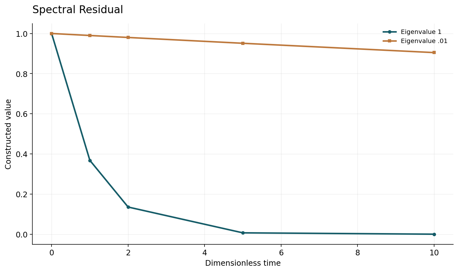
For a constructed two-mode residual with unit coefficients and eigenvalues one and0.01, the fast coefficient at time five is exp(-5), while the slow coefficient is exp(-0.05). A small training loss at a later time depends strongly on how target signal and label noise project onto those modes. Early stopping therefore cannot be chosen responsibly from eigenvalues alone; the target decomposition and validation objective matter. The example also warns against calling a slowly learned component unimportant merely because it has a small eigenvalue. A rare but scientifically important subgroup could align with that component. The spectral calculation is algebra on a fixed matrix, not evidence that a real network's eigenbasis stays fixed throughout learning.
6. A factorized scalar model makes kernel movement explicit
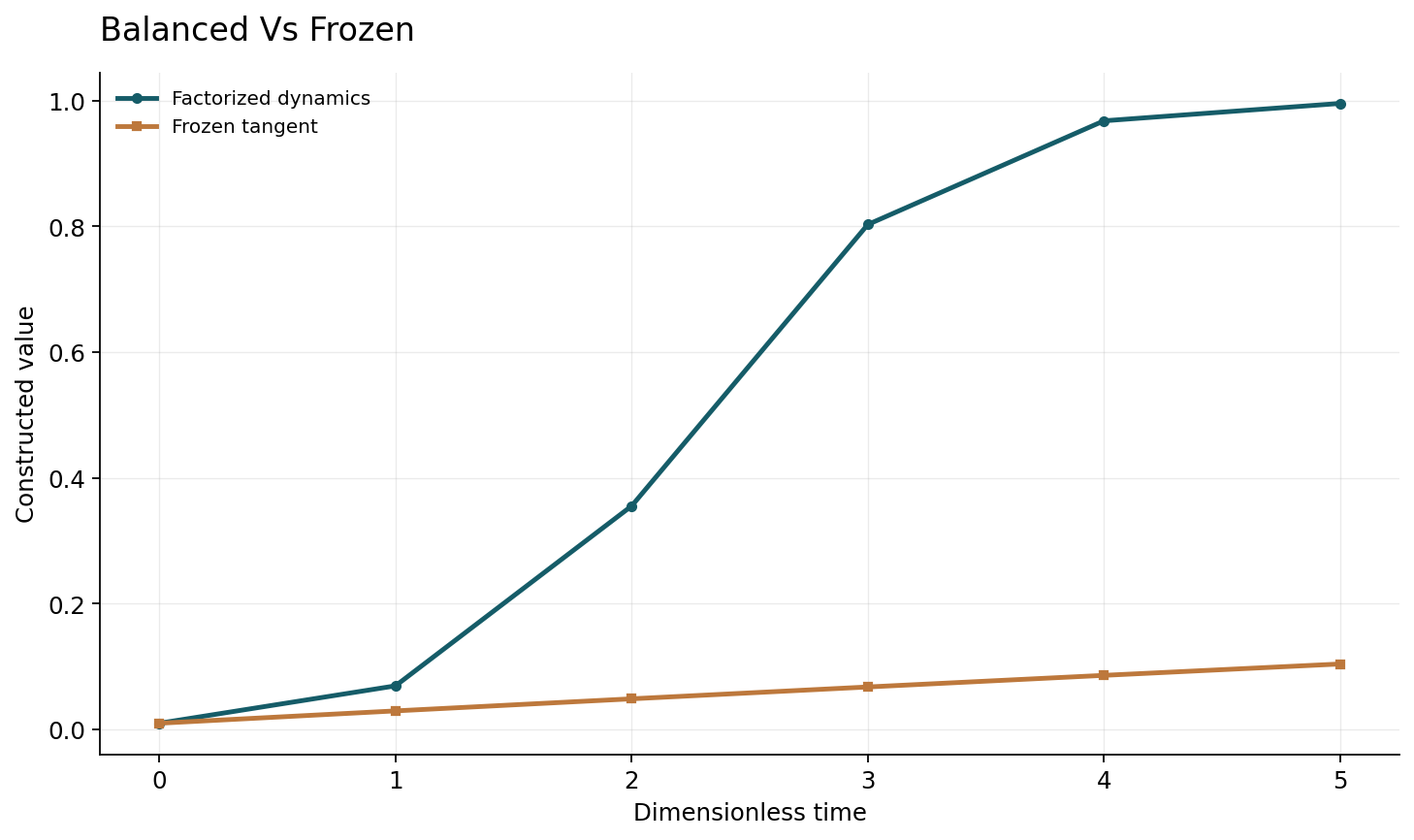
Consider f(x)=abx with one training input x=1 and target y=1. Use loss one half of(ab-1) squared and Euclidean gradient flow in a and b. Starting with a=b=s>0 preserves that equality, because the two differential equations coincide along the balanced trajectory. Writing w=a squared gives dot w=2w(1-w). Hence w(t)=1/[1+(1/w0-1)exp(-2t)] for positive initial w0.
The empirical tangent kernel on the single input is a squared plus b squared, equal to2w along the balanced trajectory. The kernel changes as the predictor approaches the target. A frozen initialization linearization instead predicts f_lin(t)=1-(1-w0)exp(-2w0 t). Both expressions are closed form and use the same initial prediction and initial tangent kernel. Their disagreement is therefore an explicit instance of a finite factorized parameterization leaving its initial tangent description. It is not a width-limit experiment or a claim about the quantitative behavior of a multilayer nonlinear network. Keeping the toy model that narrow makes it useful as a check on an argument rather than an illustration that overpromises.
7. A changing kernel does not automatically mean better features
In the scalar construction, every predictor is still a scalar multiple of x. The model has not discovered a new input direction, a compositional concept, or a transferable representation. Its tangent scale changes because the same linear function is parameterized as a product. Thus kernel drift can certify that a particular frozen approximation has changed while failing to certify an expansion of useful representational capabilities.
This distinction suggests several separate measurements. Kernel drift compares tangent similarities at chosen inputs. Functional nonlinearity compares a trained model with its initialization linearization. Representation change examines hidden activations under a stated alignment or invariance convention. Task-relevant feature learning asks whether that change improves an independently defined prediction or transfer task. None of these quantities implies all the others without additional assumptions. In particular, a large relative kernel change can be caused by a small initial norm in its denominator. Reporting absolute and normalized changes, along with the chosen probe inputs and normalization, avoids turning a convenient diagnostic into a universal scientific definition of learning.
8. Taylor remainder exposes the approximation error
For the bilinear model, the first-order expansion around(a0,b0) has an exact remainder Delta a times Delta b times x. This follows directly by expanding(a0+Delta a)(b0+Delta b)x. Small changes in each factor make the remainder second order in those changes, but whether that is negligible depends on the scale of the initial Jacobian and the desired prediction accuracy.
More generally, a Taylor-remainder bound requires a suitable Hessian control over the part of parameter space actually visited. A small Euclidean distance by itself can be uninformative if curvature is large or if a parameterization rescales that distance. Conversely, many coordinates can each change slightly while a relevant aggregate feature changes materially. A disciplined approximation claim identifies a norm, a region, a time horizon, and a bound or measured error on the predicted outputs. It should not substitute an arbitrary small percentage change in parameter norm for that statement. The exact bilinear remainder is a useful negative control because a procedure that predicts zero remainder after both factors move is demonstrably calculating the wrong object.
9. Parameterization and limits must be taken in a stated order
A width limit is a sequence of models, initializations, output normalizations, and learning rates. Changing any element can change the limiting dynamics. The inspected lazy-training and feature-learning papers make parameterization a substantive part of the theory, rather than a nuisance that can be removed from a figure caption. Finite-width behavior also need not be approximated uniformly over arbitrarily long training times by a limit proved on a fixed horizon.
One practical consequence is that experiments varying width should state how the optimizer's step size and parameter groups scale. Holding a library default learning rate fixed while changing output normalization can change the effective training regime. A second consequence concerns pretraining: a kernel description of training around one random initialization does not automatically describe fine-tuning around a learned checkpoint with structured features and different layer-wise scales. A theorem about the former can remain correct while being an unsuitable explanation for the latter. We treat those differences as questions to be tested, not as reasons to dismiss kernel theory or to claim that one limiting regime must explain every neural application.
10. Architecture-aware assumptions are not optional details
Weight sharing, normalization, recurrence, and attention create dependencies that a naive independent-layer calculation may miss. Tensor Programs II explicitly discusses when a gradient-independence shortcut is justified and when it can fail. That warning has a broader methodological implication: a limiting-kernel formula should be derived for the actual architecture and parameter sharing being evaluated, rather than copied from a superficially similar fully connected network.
The input preprocessing and output convention also matter. Bias parameters, trainable normalization scales, frozen layers, and tied embeddings determine which columns appear in the Jacobian. Omitting trainable parameters from the empirical tangent features changes the comparison model; including frozen parameters changes it in the opposite direction. A reproducible study should publish these choices and validate the Jacobian computation using finite differences or automatic-differentiation consistency checks on a small instance. The result of that validation is not a theorem about the wide limit, but it can prevent an implementation error from being misinterpreted as a scientific disagreement between nonlinear learning and kernel dynamics.
Sources: [4]
11. Training agreement is not a generalization theorem
Suppose the finite and linearized models attain nearly identical training predictions. This does not imply that their out-of-sample predictions, uncertainty, robustness, or transfer quality agree. A finite training set constrains only a restricted part of function space. A generalization claim requires a data-generating model or a well-defined test distribution, and a transfer claim needs a target task that was not used to choose the representation diagnostic.
The same caution applies to favorable training convergence. A positive minimum eigenvalue can control optimization of the stated squared-loss problem, while saying little by itself about whether the learned function matches the intended scientific target. Conversely, a fixed-kernel baseline can generalize well in a suitable problem and should not be dismissed because it does not update hidden features. The right empirical question is comparative and conditional: which procedure improves a predeclared target under matched data, computation, tuning, and evaluation? Kernel theory supplies a valuable reference model. It does not remove the need to define that target or to evaluate the costs of leaving the reference regime.
12. A reproducible analytical comparison
The supplied construction evaluates the exact balanced trajectory and the frozen prediction at selected times for w0=0.01. It records prediction error and tangent-kernel value separately. A second illustration plots two independent residual modes with eigenvalues one and0.01. All axes are dimensionless model quantities, and no curve is presented as a measured network benchmark.
The verification should check initial conditions, the closed-form differential equation, the limiting value as time grows, and agreement with a small-step numerical integrator within a declared tolerance. A deliberately incorrect frozen model using a different initial offset should fail the matched-initial-condition check. Another negative control should demonstrate that setting the tangent kernel to its final value is not the same comparison as freezing it at initialization. These controls matter because an apparently sophisticated plot can otherwise compare different models without noticing. The numerical integrator is only a consistency check for the constructed equations; its successful execution does not independently validate any of the six cited papers' proofs or practical experiments.
For the selected initial value, the nonlinear prediction at time two is about0.3555, while the matched frozen prediction is about0.0488. At time five the corresponding values are about0.9955 and0.1042. The fast improvement in the nonlinear construction follows from the increasing scalar tangent value, not from discovering a richer input representation. The gap would be interpreted incorrectly if the horizontal axes used different loss normalizations or learning-rate conventions. It would also be misleading to divide only one trajectory's residual by its own initial residual and call the resulting chart a direct output comparison. The artifact therefore retains raw predictions, residuals, and tangent values together. Such bookkeeping is simple in this example but becomes essential when comparing finite networks whose output scale, label preprocessing, or trainable layers differ. Matching those conventions is a prerequisite to interpreting a disagreement as evidence for a particular learning mechanism.
13. A study that can distinguish the competing explanations
Freeze datasets, preprocessing, architecture, parameterization, initialization seeds, trainable parameter groups, loss, and optimizer settings. Train both the finite model and its explicitly instantiated initialization linearization. Use held-out probe inputs to compute output discrepancies and kernel diagnostics throughout training, while ensuring that diagnostic sampling does not alter the training data or tuning procedure.
Vary width and scaling separately. Report the learning-rate and compute budgets, failed runs, and sensitivity to the probe set. Add at least one target that requires useful representation change under a justified task model, and at least one control where a fixed feature map is sufficient. For transfer, separate the data used to train the representation from the data used to evaluate and select the downstream predictor. A result supporting feature learning should connect a functional or representation change to the predeclared target, rather than merely showing that a matrix moved. The remaining limitations should identify which architectures, training horizons, and data distributions were not tested. Such an evaluation can challenge a proposed explanation while leaving a conditional wide-limit theorem intact.
14. What a defensible interpretation would say
The most useful conclusion is not that neural networks are kernels or that kernel theory cannot explain neural networks. It is that a finite network has an exact instantaneous tangent description under specified dynamics, and a fixed tangent approximation is an additional claim whose accuracy and scientific relevance must be established. Different parameterizations can lead to different limits, and different tasks can benefit from different kinds of learned structure.
The scalar construction sharpens the boundary: leaving the initial kernel regime can happen without discovering any richer input feature. Conversely, an accurate kernel approximation can be valuable even when it is not an account of transfer learning. Open questions include how to identify diagnostics that predict task-relevant representation change, how to compare limits across realistic optimizer choices, and how to allocate finite computation between useful feature adaptation and stable optimization. Answering those questions requires matched experimental designs and clear definitions. The analytical examples here provide checks on the definitions and arithmetic; they do not supply new empirical evidence about which mechanism dominates contemporary large-model training.
Core equations and definitions
(1) Exact chain rule for differentiable outputs, loss(1/2)||f-y||² and Euclidean gradient flow; no width limit.
(2) Exact dynamics of the initialization-linearized squared-loss model on the fixed training set.
(3) Author-constructed balanced model f(x)=abx at x=y=1 with a=b>0.
(4) Matched frozen initialization tangent prediction for the constructed scalar model.
(5) Exact first-order Taylor remainder for a bilinear model; not a bound for arbitrary networks.
Constructed analytical figures
Comparison and reporting contract
| Diagnostic | What it measures | What it does not establish alone |
|---|---|---|
| Tangent-kernel drift | Change in local parameter-to-output geometry | Useful new representation |
| Linearization discrepancy | Departure from initialization Taylor model | Better generalization |
| Hidden representation movement | Change under a stated alignment convention | Causal contribution to target performance |
| Held-out transfer benefit | Task-specific usefulness under an evaluation protocol | Universal superiority of a training regime |
Evaluation protocol
- Freeze initialization outputs and Jacobian for matched comparisons.
- State loss normalization and optimizer metric.
- Test trainable/frozen parameter groups explicitly.
- Check Jacobians on a small instance.
- Vary width and scaling separately.
- Evaluate finite and initialization-linearized predictors under matched budgets.
- Measure held-out function and representation diagnostics.
- Separate transfer selection from representation training data.
- Retain failures and probe-set sensitivity.
- Distinguish constructed equations from empirical network evidence.
Limitations
- No deep neural network or published benchmark is newly trained here.
- The exact tangent identity uses Euclidean gradient flow and squared loss.
- The scalar example remains linear in the input and cannot demonstrate rich representation learning.
- Source proofs were not independently verified; only identified source scope was inspected.
- No universal parameterization or optimizer recommendation follows from these examples.
Open research questions
- Which diagnostics predict useful feature adaptation rather than merely kernel movement?
- How should wide-limit comparisons incorporate realistic optimizer metrics and pretraining?
- When does finite computation favor leaving an initialization tangent regime?
Evidence and its boundaries
- The tangent kernel is finite and evolving before a specified infinite-width limit makes it constant.
- [1] — Only the inspected source scope is used; no source benchmark or proof is claimed as independently reproduced. Inspected: Original abstract and PDF introduction/NTK formulation.
- The studied wide-network limit is governed by an initialization linearization under stated dynamics.
- [2] — Only the inspected source scope is used; no source benchmark or proof is claimed as independently reproduced. Inspected: Original abstract and PDF first-order linearization description.
- Lazy behavior depends on scaling and is not simply a synonym for parameter count.
- [3] — Only the inspected source scope is used; no source benchmark or proof is claimed as independently reproduced. Inspected: Original abstract and PDF introduction/scaling motivation.
- Architecture-specific dependencies qualify limiting-kernel calculations.
- [4] — Only the inspected source scope is used; no source benchmark or proof is claimed as independently reproduced. Inspected: Original abstract, architecture and gradient-independence qualification.
- Some parameterizations retain feature learning at infinite width, unlike the stated standard/NTK regimes.
- [5] — Only the inspected source scope is used; no source benchmark or proof is claimed as independently reproduced. Inspected: Original abstract and parameterization/feature-learning scope.
- The measure-valued many-particle gradient-flow formulation is a distinct conditional construction.
- [6] — Only the inspected source scope is used; no source benchmark or proof is claimed as independently reproduced. Inspected: Original abstract and many-particle measure/initialization qualifications.
References
- Neural Tangent Kernel: Convergence and Generalization in Neural Networks
Arthur Jacot, Franck Gabriel, Clément Hongler. NeurIPS2018 (2018). https://arxiv.org/abs/1806.07572Source scope
Original abstract and PDF introduction/NTK formulation.
- Wide Neural Networks of Any Depth Evolve as Linear Models Under Gradient Descent
Jaehoon Lee, Lechao Xiao, Samuel S. Schoenholz, Yasaman Bahri, Roman Novak, Jascha Sohl-Dickstein, Jeffrey Pennington. NeurIPS2019 (2019). https://arxiv.org/abs/1902.06720Source scope
Original abstract and PDF first-order linearization description.
- On Lazy Training in Differentiable Programming
Lénaïc Chizat, Edouard Oyallon, Francis Bach. NeurIPS2019 (2019). https://arxiv.org/abs/1812.07956Source scope
Original abstract and PDF introduction/scaling motivation.
- Tensor Programs II: Neural Tangent Kernel for Any Architecture
Greg Yang. arXiv:2006.14548 (2020). https://arxiv.org/abs/2006.14548Source scope
Original abstract, architecture and gradient-independence qualification.
- Feature Learning in Infinite-Width Neural Networks
Greg Yang, Edward J. Hu. ICML2021 / arXiv version3 (2021). https://arxiv.org/abs/2011.14522Source scope
Original abstract and parameterization/feature-learning scope.
- On the Global Convergence of Gradient Descent for Over-parameterized Models using Optimal Transport
Lénaïc Chizat, Francis Bach. NeurIPS2018 (2018). https://arxiv.org/abs/1805.09545Source scope
Original abstract and many-particle measure/initialization qualifications.