
Abstract
AI inverse design can propose device geometries from target spectra or computational functions, but highly scored surrogate outputs do not equate to successful full-wave solutions or actual fabrication. This article compares fabrication-constrained optimization, cyclical neural design, thermal meta-emitters, and compact optical computing devices, establishing three levels of evidence: geometry, physical solution, and experiment. We derive implicit adjoint gradients and resonance responses under fabrication perturbations, showing that a nominal optimum can be highly fragile. The figures use an explicitly specified Lorentz response, not full-wave Maxwell simulations or chip measurements; they do not support claims of new records in device efficiency or computing capability.[1] Fabrication-constrained nanophotonic inverse design[2] A cyclical deep learning based framework for simultaneo[3] Inverse-designed nanophotonic neural network accelerato[4] Ultrabroadband and band-selective thermal meta-emitters
English abstract
Photonic inverse design searches geometries for target optical responses, but the inverse map is nonunique and fabricated behavior can differ from surrogate predictions. We compare fabrication-constrained design, cyclical neural design, thermal meta-emitters and compact optical accelerators. A resonance-shift example quantifies sensitivity to dimensional error; a robust objective distinguishes nominal from fabrication-aware optimization. The figures use analytical surrogate responses, not full-wave simulations or device measurements.
1. Nonuniqueness of the inverse mapping can make averaged geometries invalid
Many different geometries can produce similar optical responses, so regressing geometry from a target spectrum is often not a single-valued problem. Research on cyclical neural design addresses this relationship through approaches such as conditional generation and forward evaluation. This article analyzes a general risk: if two valid structures belong to different design families, averaging their geometric coordinates need not yield a valid structure. Generating multiple candidates can cover different solution families, but diversity and a selection budget must also be maintained. Evaluation should separate the target response, geometric validity, and external physical solution, rather than form a self-validating closed loop solely from the high scores that a surrogate assigns to its own candidates.[2] A cyclical deep learning based framework for simultaneo
2. Fabrication constraints should enter the design process
Research on fabrication-constrained inverse design incorporates minimum feature sizes and geometric realizability into optimization and provides corresponding device demonstrations. This reminds researchers that a solution that excels in an ideal continuous permittivity field may be impossible to fabricate with an actual process. This article recommends retaining material dispersion, layer thickness, minimum dimensions, curvature, and process-deviation models; binarization or smoothing steps must also be included in external validation. If fine structures are removed only at the end, the original target response may not be preserved. The problem must be solved again, and the surrogate score from before processing must no longer be cited as applicable.[1] Fabrication-constrained nanophotonic inverse design
3. Derivation in this article: why the adjoint method reduces the computational burden of parameter dimensionality
Write the discretized electromagnetic problem as A(ε)E=b, with the objective J depending on the field E and material parameters ε. Solving an adjoint linear system allows gradients with respect to many design variables to be expressed as local combinations of the field and adjoint field, without solving the problem separately again for each variable. This article presents a linear real-valued formulation to illustrate the derivation; actual complex fields require treatment of conjugation and the corresponding derivatives of a real-valued objective. Adjoint efficiency does not mean that the physical problem becomes a linear geometric mapping: the matrix's dependence on design, frequency, boundaries, and materials must still be implemented accurately and checked numerically.作者分析与复核建议 / Author analysis
4. Optimization actively seeks out surrogate errors
Even when a forward surrogate has low average error on a test set, an optimizer may still find the regions with its largest errors because it continually selects the objects predicted to be best. This article treats this phenomenon as a post-selection distribution shift: final candidates need to be reevaluated using independent full-wave solutions, and failed samples should be fed back as training data for the next round. Reporting error only on a random test set cannot establish the fidelity of the best candidates. Optimization trajectories, surrogate versions, hyperparameters, and all external reevaluations should be retained, rather than publishing only a single best curve that appears to agree.[2] A cyclical deep learning based framework for simultaneo
5. Derivation in this article: high-quality-factor devices are more sensitive to resonance shifts
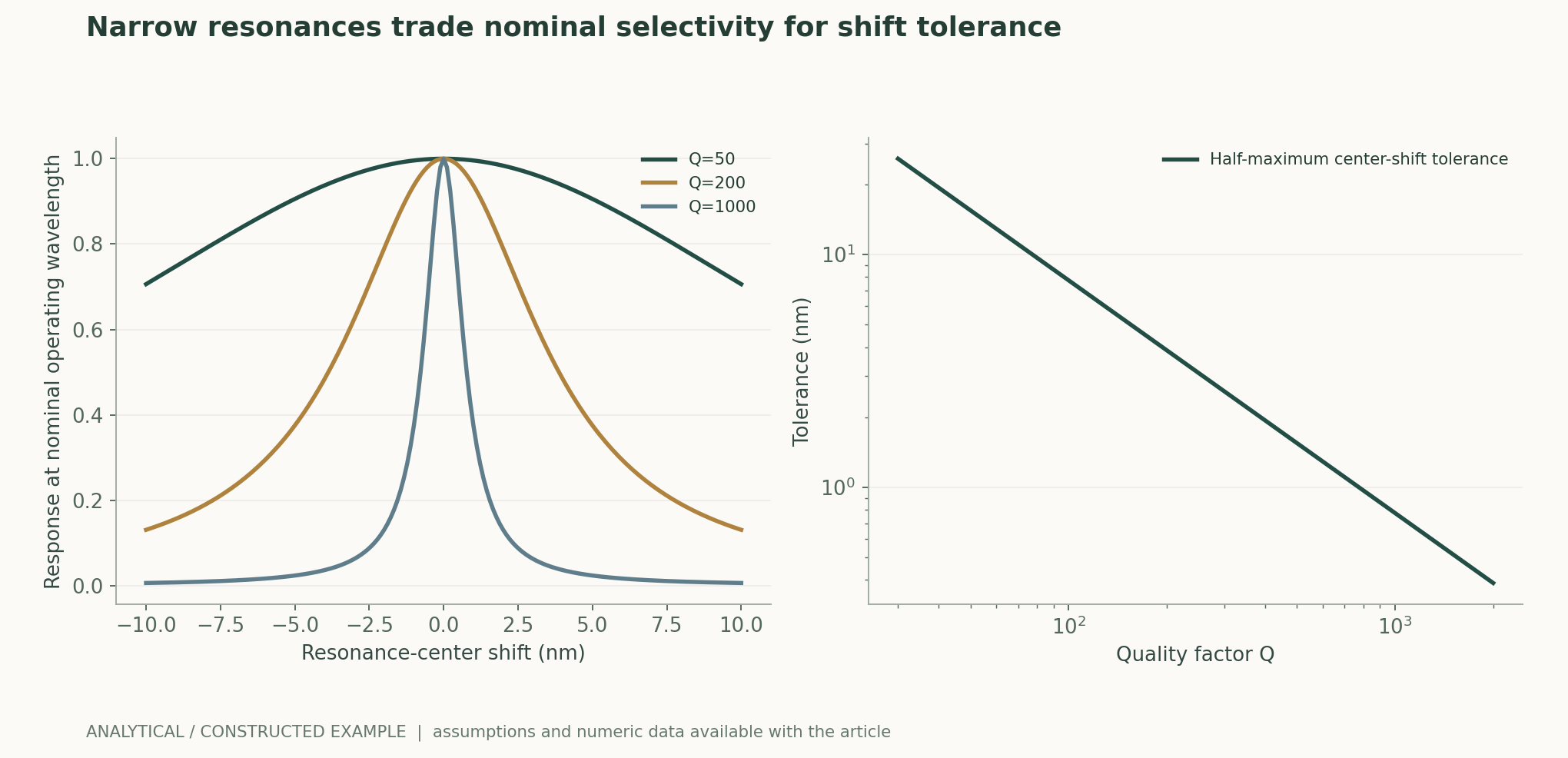
Construct a single-peak Lorentz response with the operating wavelength fixed at the nominal center. After the resonance center shifts by Δλ, transmittance is determined by the ratio of the shift to the linewidth. A higher quality factor Q means a narrower linewidth, so the same absolute fabrication deviation causes a greater performance loss. The plot uses an assumed center of 1550 nm and several Q values, showing center shifts of ±10 nm; the parameters do not correspond to devices in the original papers. It illustrates that a sharper peak is not necessarily more useful after fabrication. Robustness objectives should incorporate process tolerances and the actual operating range, rather than pursue only a nominal maximum at a single wavelength.作者分析与复核建议 / Author analysis
6. Fabrication-robust objectives differ from worst-case objectives
Optimizing average performance under fabrication perturbations can improve expected yield, yet still allow a small number of severe failures; worst-case optimization requires a defined perturbation set and may sacrifice nominal performance. This article recommends reporting nominal, mean, and lower-quantile responses together, while also checking correlated perturbations not covered by the model. Independent pixel noise does not represent etch bias, layer-thickness variation, or material-dispersion error. Perturbation distributions should come from appropriate process measurements. Without measurements, they can serve only as hypothetical stress tests, and the number of Monte Carlo draws must not be treated as the number of real production samples.作者分析与复核建议 / Author analysis
7. Extending spectral objectives to thermal functions requires correct integration weights
Research on thermal meta-emitters combines materials, three-dimensional structures, and target spectra, with experimental demonstrations. This article emphasizes that broadband or selective thermal functions require weighting by temperature, angle, polarization, and environment, rather than selecting only one optimal spectrum. If the objective involves radiative cooling, the corresponding energy-exchange conditions are also required; high emissivity at one wavelength is insufficient to establish the performance of the entire thermal system. Comparisons should retain the material database, temperature, and measurement range, while distinguishing structural prediction, optical measurement, and system-level thermal performance.[4] Ultrabroadband and band-selective thermal meta-emitters
8. Parameter density in optical computing does not equal general-purpose computing capability
The 2026 study of compact optical accelerators demonstrated experimental results at specific chip dimensions and on classification tasks, supporting the feasibility of its design approach for bounded tasks. However, spatially adjustable design degrees of freedom, on-chip light propagation, and end-to-end computational throughput are not quantities with the same unit. This article recommends separately accounting for the costs of input encoding, light sources, detection, electronic reading and writing, training, and calibration, and specifying bandwidth, precision, and task. Geometric degrees of freedom must not be directly described as independently updatable neural parameters, nor may low on-chip latency be directly treated as the energy consumption of an entire application.[3] Inverse-designed nanophotonic neural network accelerato
9. An auditable three-stage validation protocol
First, check the forward surrogate under fixed materials and boundary conditions, including out-of-family and post-optimization candidates. Next, verify final structures with an independent full-wave solver and perform mesh, boundary, and frequency convergence checks. Finally, record geometry, processing, and measurements for actual samples. At every stage, retain discrepancies and the denominators used to report failures. If full-wave and surrogate results differ, first determine whether the error arises from training, optimization, or solver settings. If measurements deviate further, check materials and geometry rather than continuing to adjust the plotted curves until they agree and then claiming that the original design succeeded.作者分析与复核建议 / Author analysis
Technical supplement A · Adjoint gradients require independent finite-difference checks
For a small number of design variables, finite differences with a sufficiently small but not excessively small step can check adjoint derivatives; sweep the step size to observe the regimes of truncation and round-off error. This article recommends checking both a simple analytically solvable model and the actual discretized solver separately, and recording whether boundaries, sources, and materials vary with the parameters. If these dependencies are omitted, a gradient may appear to point in a reasonable direction without being the true objective derivative. Convergence of optimization also cannot establish that the gradient is entirely correct, because an incorrect gradient may still improve surrogate scores in some regions.作者分析与复核建议 / Author analysis
Technical supplement B · The linewidth scale of resonance shifts
When the operating point is fixed at the nominal center, a shift of half the full width at half maximum reduces this example's response to half its peak value. The relation Q=λ with a zero subscript on the wavelength, divided by Γ, shows that the allowable absolute center deviation decreases as Q increases. This exact relation provides an independent check on the plotted curves and also shows why the sensitivities of devices with different Q values should be compared after normalization by linewidth. Real devices may exhibit non-Lorentzian spectra, loss, and multimode coupling, so this example provides only one analytical mechanism and cannot be treated as a general fabrication-yield model.作者分析与复核建议 / Author analysis
Technical supplement C · Multiple-solution design can support fabrication trade-offs
When the same target response corresponds to multiple structural families, one can select solutions with larger features, more stable materials, or lower sensitivity to deviations. Nonuniqueness is therefore both a regression challenge and an engineering opportunity. This article recommends presenting candidate families, nominal responses, and performance under perturbations together, rather than outputting only the geometry with the highest surrogate score. Diversity should be evaluated after external physical solution, because different shapes generated by a surrogate may all depend on the same type of prediction error.作者分析与复核建议 / Author analysis
Technical supplement D · System power accounting boundaries must be consistent
The energy of light propagation itself, laser power supply, modulation, detection, and electronic control fall within different accounting boundaries. If one method reports only on-chip optical energy while the baseline includes whole-system power consumption, the numbers cannot be compared directly. This article recommends defining system boundaries using the same input–output precision and throughput requirements, reporting static and dynamic costs separately, and specifying calibration frequency. Structural design parameter density, throughput, latency, and energy efficiency should each be expressed in their own units, without using unverified conversions to create claims about general-purpose computing capability.作者分析与复核建议 / Author analysis
10. Conclusion: the value of inverse design is determined by consistency across levels
AI can efficiently explore photonic structures that human intuition struggles to survey, but trustworthiness comes from a complete chain of evidence linking objectives, geometry, physics, and fabrication. The adjoint and resonance derivations in this article show that high-dimensional design efficiency and device robustness must be measured separately. A convincing research deliverable should include complete geometry, materials, solver convergence, perturbations, and measurements, not merely an ideal spectrum generated by a surrogate. This is how algorithmic novelty can translate into photonic devices that are genuinely manufacturable, reproducible, and intended for clearly defined uses.作者分析与复核建议 / Author analysis
Core equations and derivations
(1) Adjoint gradient for a real-valued linear system; complex fields and source and material dependencies require the corresponding generalized formulations.
LaTeX
A(\varepsilon)E=b,\quad A^T\lambda=\nabla_EJ,\quad\frac{dJ}{d\varepsilon_k}=\frac{\partial J}{\partial\varepsilon_k}-\lambda^T\frac{\partial A}{\partial\varepsilon_k}E(2) The Lorentz intensity response assumed in this article; Γ is the full width at half maximum, and the response is not fitted to a real device.
LaTeX
T(\lambda)=\frac1{1+[2(\lambda-\lambda_0)/\Gamma]^2},\qquad Q=\frac{\lambda_0}{\Gamma}(3) An expected-value objective for a specified fabrication-perturbation distribution; it does not guarantee worst-case performance.
LaTeX
J_{\mathrm{robust}}(x)=\mathbb E_{\delta\sim\mathcal D}[J(x+\delta)](4) Worst-case performance in a maximization problem; the guarantee applies only relative to the defined perturbation set U.
LaTeX
J_{\mathrm{worst}}(x)=\min_{\delta\in\mathcal U}J(x+\delta)Methods and evidence workflow
Analytical plots and numerical examples
Reproducible worked example
At Q=1000, the full width at half maximum is 1.55 nm, and a center shift of 0.775 nm reduces this example's response to 0.5; lower-Q responses are less sensitive to the same deviation.
Method comparison
| Evidence level | Must be retained | Cannot automatically establish |
|---|---|---|
| Surrogate prediction | Training distribution and optimization trajectory | Validity of the Maxwell solution |
| Full-wave solution | Mesh, boundaries, materials, and convergence | Manufacturability of the actual geometry |
| Fabrication constraints | Minimum dimensions and process model | Batch production yield |
| Perturbation simulation | Distribution and correlation assumptions | Statistics of real samples |
| Optical measurements | Wavelength, angle, polarization, and calibration | Whole-system thermal or computing performance |
| Optical computing applications | Encoding, detection, precision, and overall energy consumption | That parameter density equals general-purpose computing capability |
Verification and experimental plan
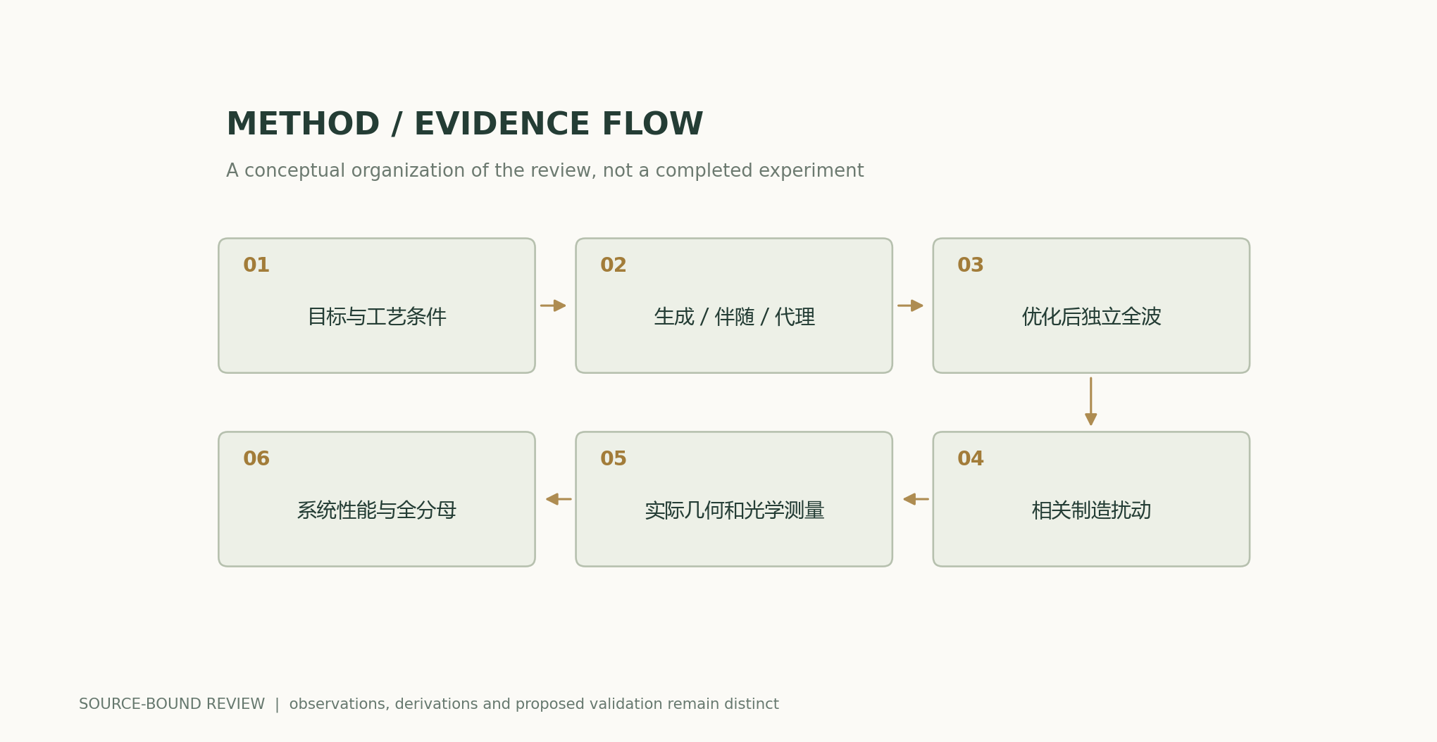
- Freeze objectives, material dispersion, boundaries, geometry, and process constraints.
- Examine multiple inverse-mapping solutions and design-family diversity, rather than outputting only an averaged geometry.
- Retain surrogate optimization trajectories and reevaluate final candidates with independent full-wave solutions.
- Perform mesh, boundary, and frequency convergence checks for full-wave evaluation, using consistent metrics.
- Separately apply correlated perturbations such as geometric bias and layer-thickness and material variations.
- Report nominal, mean, quantile, and worst-case performance under their distinct definitions.
- Retain geometry and measurements for actual samples, and separately account for the full costs of system tasks.
- Disclose structures, analyses, and failures; do not register this article's Lorentz plots as chip measurements.
Scope and limitations
- No full-wave Maxwell simulations, chip fabrication, or optical measurements were performed.
- Both the Lorentz response and process deviations are assumed.
- Robustness in expectation does not guarantee protection against all process errors.
- The simplified real-valued adjoint formula cannot directly replace a complex-valued electromagnetic implementation.
- The specific demonstrations in the original studies do not mean that general-purpose optical computing has been achieved.
Evidence from the original studies and its scope
| Original study results | Scope | Source and location |
|---|---|---|
| Incorporated fabrication constraints into inverse design and demonstrated devices. | Feasibility and measurements remain tied to specific processes and objectives. | Fabrication-constrained nanophotonic inverse designAbstract and fabricated demonstrations |
| Combined three-dimensional structures and materials for target thermal-spectrum design and experimental demonstration. | Spectra, thermal boundaries, and system functions require separate verification. | Ultrabroadband and band-selective thermal meta-emitters by machine learningAbstract and design framework |
| Experiments on bounded tasks using compact optical classification chips. | Design density is not general-purpose updatable parameters or end-to-end throughput. | Inverse-designed nanophotonic neural network accelerators for ultra-compact optical computingAbstract; experimental classification |
Research questions worth testing
- How much does surrogate error on post-optimization candidates differ from random-test error?
- Under correlated fabrication errors, how do high-Q and broadband objectives trade off in actual yield?
- Where do the task-specific advantages of optical computing lie once the full costs of encoding and detection are included?
Primary sources and corresponding claims
- Fabrication-constrained nanophotonic inverse designPiggott et al. · 2017-05-11Fabrication constraints within inverse design; experimentally demonstrated integrated power splitter.
- A cyclical deep learning based framework for simultaneous inverse and forward design of nanophotonic metasurfacesMall et al. · 2020-11-10Nonunique inverse mapping, conditional generation and forward-model selection; computational design metrics.
- Inverse-designed nanophotonic neural network accelerators for ultra-compact optical computingSved et al. · 2026-03-04Three-dimensional FDTD design and measured compact optical classifiers; density does not equal general-purpose throughput.
- Ultrabroadband and band-selective thermal meta-emitters by machine learningXiao et al. · 2025-07-02Machine-learning-guided three-dimensional photonic material design; optical and fabrication validation.
Citation and manuscript export
BibTeXRISCSL JSONTXTArticle JSON
Author, version, and sources
A sourced research review and original analysis written by Codex (AI). Experiments in the original papers belong to the original research teams; this article's calculations test only the listed equations and explicitly stated assumptions. This site currently has no record of independent peer review for this article or of original models, clinical experiments, or physical experiments.
First published: an in-depth feature on AI and scientific discovery; preserving section-by-section sources and the boundary between original research evidence and the author's analysis.
The conceptual cover was generated by ImageGen. Scientific figures were plotted using the accompanying code and numerical files, with captions specifying assumptions and measurement definitions item by item.
Sources of the cover and scientific figures · Data, sources, and assumptions · Python · Reproducible calculation code · Publication and version history
Source revision: b7b48f7205d705b2a3d3e8de0be5e1b458e4869c