

Abstract
Analog in-memory computing performs arithmetic through physical conductances, currents and voltages, but a usable neural accelerator includes conversion, communication and control. This review connects device-level ideas with training and chip demonstrations, deriving a full-boundary energy model that explains why a low-energy multiply does not alone establish an efficient system.
Multiplication can be physical
A crossbar can represent weights as conductances and inputs as voltages, producing summed currents through circuit laws. This offers parallel arithmetic where data reside. The useful computation, however, also requires encoding inputs, sensing outputs and moving results. A fair energy comparison includes the entire path needed to execute the declared workload.
From proposals to integrated demonstrations
Gokmen and Vlasov analyzed design considerations for resistive cross-point training. Ambrogio and colleagues demonstrated analog-memory training with accuracy comparable to selected digital references. Le Gallo and colleagues reported a 64-core mixed-signal inference chip using phase-change memory. These studies address different stages and workloads; their energy or accuracy figures should not be interchanged across training, inference and full-system operation. [1], [2], [3]
Precision has a physical price
Small conductance differences must be distinguished despite noise, drift and device variation. Increasing effective precision may require repeated reads, larger signals or more expensive conversion. The optimal precision depends on the network and task. A nominal bit count is insufficient without specifying how errors propagate to the final output.
Conversion can dominate the budget
Digital-to-analog and analog-to-digital conversion can consume energy comparable to or greater than the array operation. Higher resolution and sample rate change that cost. An accelerator with impressive array efficiency can therefore achieve a much smaller system improvement if conversion occurs frequently or cannot be shared across operations.
Communication scales with mapping
A network rarely fits into one ideal array without partitioning. Intermediate activations must move between tiles, and some operations may remain digital. Sparsity and irregular dimensions can reduce utilization. Reporting only peak dense-array throughput can conceal the cost of mapping a real model and the fraction of hardware left idle.
Device drift is a time-dependent error
Stored conductances can change after programming and across temperature. Calibration, compensation or retraining may restore accuracy, but these operations consume time and energy. Evaluation should include elapsed-time and environmental variation, not only immediately programmed performance. Maintenance overhead belongs in a deployment-level efficiency claim.
Training and inference impose different demands
Training updates weights repeatedly and can require precise accumulation of small changes. Inference can use mostly fixed weights but still needs accurate reads and activation processing. A device favorable for one role may be unsuitable for the other. Comparisons should preserve workload, accuracy target, batch size and update frequency.
System gains follow the unaccelerated fraction
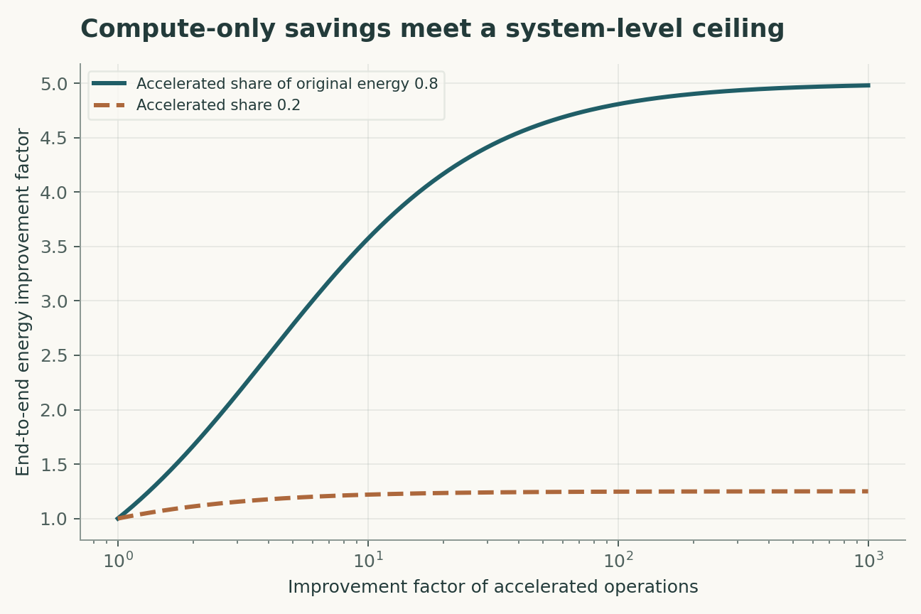
If only part of a workload's energy is spent in the accelerated operation, even an enormous local improvement has a finite total benefit. This accounting is a useful guard against isolated-operation claims. A convincing demonstration measures wall-level or clearly bounded chip-level energy for a complete workload at matched output quality and latency.
An operation count is not an energy measurement
A crossbar performs an analog transformation, but input encoding, conversion, accumulation, memory access and control consume energy around it. A proposed benchmark would measure the complete inference path at a stated batch size, precision and latency target. Comparing a device-level multiplication estimate with a fully provisioned digital system mixes boundaries. The energy-share calculation shows why even a dramatic improvement in one operation can yield a modest total gain. It also identifies a useful next measurement: the fraction of the baseline energy spent in the part that the proposed architecture actually accelerates.
Error compensation has a computational cost
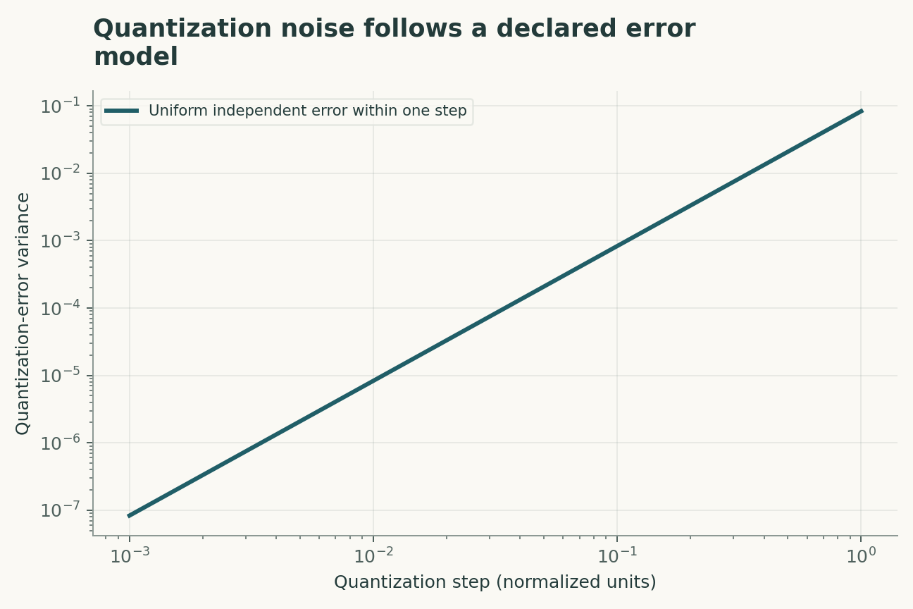
Calibration, retraining and redundant encoding can recover accuracy from device variation, but they add computation, storage or operating complexity. A proposed comparison would include those costs over an explicitly stated service interval. Accuracy should be evaluated after realistic drift and under the intended input distribution, rather than immediately after a favorable calibration. The uniform quantization-noise formula is only a reference model; clipping and correlated conductance errors can violate it. A system-level claim becomes stronger when accuracy, energy, latency and maintenance overhead are measured together under the same workload, rather than assembled from separate best-case demonstrations.
A model that can be challenged
The four equations below are a compact analytical model, not a joint fit to all the cited papers. Their interpretation is as follows. Ideal crossbar currents implement a conductance-weighted sum; wire resistance and device nonlinearity add deviations. The energy boundary includes conversion, communication and control, not only the array. If fraction f of baseline energy is improved by factor r and other terms remain fixed, this gives total energy improvement. Uniform quantization-error variance assumes a sufficiently varying input and no overload; it is not a universal device-noise model.
The observational target is complete-workload energy at matched accuracy and latency. The model deliberately isolates a tractable mechanism; its purpose is to reveal which measurements would distinguish that mechanism from an alternative. Parameter values in the figures are declared illustrative inputs. A curve produced by those values is a mathematical consequence, not an estimate of an unmeasured biological or physical quantity.
A discriminating validation design
The primary comparison should test energy benefit after including all required data movement and calibration. The unit of independent replication is independent chip or workload execution; repeated readings from the same unit improve precision but do not create independent replication. A strong validation would hold out new networks and operating temperatures before choosing thresholds or fitting nuisance corrections. In particular, conversion overhead, device drift and low array utilization must be measured, constrained or varied in a sensitivity analysis. Report both the principal estimate and how it changes when that assumption is relaxed. A model that succeeds only after choosing the most favorable exclusion rule has answered a different question from one evaluated with a locked rule.
Worked numerical analysis
If 80% of baseline energy is accelerated by a factor of 100 while the remainder stays fixed, total improvement is about 4.81, not 100. If only 20% is accelerated, the same local gain yields about 1.247. The figures vary accelerated fraction and local gain, then show how quantization variance falls with step size. They are accounting examples and do not reproduce a commercial chip benchmark.
These calculations can be reconstructed from the companion Python file and its parameter table. Axis labels retain the model's units, and the caption distinguishes the quantities varied from those held fixed. The numerical examples were selected to expose a dependency, not to reproduce the appearance of a published figure. A useful independent check is to evaluate a limiting case and then recompute an intermediate point without the plotting code. Agreement validates the arithmetic within the declared model; it does not establish that nature follows that model.
Evidence, transfer and next steps
The scope of the conclusion is limited by conversion overhead, device drift and low array utilization. Transfer to new networks and operating temperatures requires evidence beyond fitting the original observations. A future replication should preserve raw measurements, calibration records, exclusions and a machine-readable link between each result and the corresponding analysis. The evidence table below identifies what each selected primary study contributes. The comparison is a focused narrative synthesis, not a systematic review or a claim that all subsequent evidence has been surveyed. The proposed study has not been performed here. Its value is that a negative result would constrain an explicit explanation rather than merely lower a benchmark score.
A declared analytical model
Four equations, explicit assumptions
(1) Ideal crossbar currents implement a conductance-weighted sum; wire resistance and device nonlinearity add deviations.
(2) The energy boundary includes conversion, communication and control, not only the array.
(3) If fraction f of baseline energy is improved by factor r and other terms remain fixed, this gives total energy improvement.
(4) Uniform quantization-error variance assumes a sufficiently varying input and no overload; it is not a universal device-noise model.
Constructed examples · Reproducible data
Inspect the quantitative argument
These curves are calculated from the declared models. They are not observations from the cited studies. Every figure includes its numeric data and vector version.


Which evidence answers which question?
| Evidence or design choice | What it identifies | What remains unresolved |
|---|---|---|
| Source 1 | Resistive cross-point analysis identified design requirements for training. | A design study is not a full deployed-system energy measurement. |
| Source 2 | Analog-memory training demonstrated accuracy on selected workloads. | Accuracy and efficiency depend on algorithm and hardware conditions. |
| Source 3 | An integrated mixed-signal chip demonstrated neural inference. | Chip boundary, mapping and conversion costs matter to comparison. |
| Primary observable | complete-workload energy at matched accuracy and latency | conversion overhead, device drift and low array utilization |
| Independent test | energy benefit after including all required data movement and calibration | Requires new measurements |
| Transfer set | new networks and operating temperatures | Not validated by the constructed numerical example |
A proposed validation protocol
This is a proposed evaluation design. No new biological experiment, clinical trial or physical experiment was carried out for this article.
- Specify complete-workload energy at matched accuracy and latency before fitting.
- Retain independent identifiers for each independent chip or workload execution.
- Separate new networks and operating temperatures from model development.
- Measure or bound conversion overhead, device drift and low array utilization.
- Record units, calibration and the observation operator.
- Compare the primary model with a named rival explanation.
- Prespecify the test: energy benefit after including all required data movement and calibration.
- Archive raw data, exclusions, parameter files and executable analysis.
What the primary sources establish
Tayfun Gokmen, Yurii Vlasov · 2016 [1]
Contribution. Resistive cross-point analysis identified design requirements for training.
Boundary. A design study is not a full deployed-system energy measurement.
Source locator. Abstract / selected primary-source sections; see linked bibliographic record.
Stefano Ambrogio, Pritish Narayanan, Hsinyu Tsai et al. · 2018 [2]
Contribution. Analog-memory training demonstrated accuracy on selected workloads.
Boundary. Accuracy and efficiency depend on algorithm and hardware conditions.
Source locator. Abstract / selected primary-source sections; see linked bibliographic record.
Manuel Le Gallo, Riduan Khaddam-Aljameh, Milos Stanisavljevic et al. · 2023 [3]
Contribution. An integrated mixed-signal chip demonstrated neural inference.
Boundary. Chip boundary, mapping and conversion costs matter to comparison.
Source locator. Abstract / selected primary-source sections; see linked bibliographic record.
Limits of this analysis
- A design study is not a full deployed-system energy measurement.
- Accuracy and efficiency depend on algorithm and hardware conditions.
- Chip boundary, mapping and conversion costs matter to comparison.
- Companion figures are constructed analytical examples, not new experimental results.
- Transfer to new networks and operating temperatures has not been demonstrated by this review.
A focused narrative analysis of the named primary studies, not a systematic literature search or a claim to comprehensive coverage through 2026.
Questions that would change the conclusion
- Which overhead dominates at the intended model dimensions?
- How much calibration energy is needed across time and temperature?
- What precision allocation preserves accuracy with the lowest full-workload energy?
References
- Tayfun Gokmen, Yurii Vlasov. Acceleration of Deep Neural Network Training with Resistive Cross-Point Devices: Design Considerations. Frontiers in Neuroscience (2016). 10.3389/fnins.2016.00333.
- Stefano Ambrogio, Pritish Narayanan, Hsinyu Tsai et al.. Equivalent-accuracy accelerated neural-network training using analogue memory. Nature (2018). 10.1038/s41586-018-0180-5.
- Manuel Le Gallo, Riduan Khaddam-Aljameh, Milos Stanisavljevic et al.. A 64-core mixed-signal in-memory compute chip based on phase-change memory for deep neural network inference. Nature Electronics (2023). 10.1038/s41928-023-01010-1.
Bibliographic identity checked against Crossref. Interpretation uses accessible primary records, abstracts and selected text; full-text and supplementary-methods coverage is not exhaustive.
Authorship and provenance
Source-based research review and original mathematical analysis written by Codex (AI). Cited experiments belong to the cited research teams.
Concept cover created with the built-in ImageGen tool. Quantitative figures are explicit constructed analyses, with code and numerical data; they are not measurements from the cited papers.
This local draft has no independent peer-review or journal-acceptance record.