
Scientific Deep Learning / DEEP LEARNING III
Forecasts Must Respect the Clock: Temporal Leakage and Evaluation
Forecast validity depends on record availability, window support and selection history before architecture.
English original. Translations of this new review are not yet available.

Abstract
An accurate retrospective estimate is not necessarily a valid forecast. This review formalizes information availability at a forecast origin and separates event time from arrival time. A stationary Gaussian autoregression gives exact valid forecast variances and smaller, invalid future-assisted variances. An interval audit enumerates windows whose targets cross a nominal split when only window start times are used. These controls are accompanied by reproducible code and two numerical figures, not newly trained forecasting benchmarks. Six primary model records provide context for recurrent, attention-based, linear and patching approaches. The proposed protocol covers normalization, revised data, cross-series availability, hyperparameter selection, missingness and prospective replay, preserving the distinction between a modeling gain and an expanded information set.
In this paper
- 1. A forecast is defined by what was available
- 2. Architecture papers answer a different question
- 3. Event time and availability time are not identical
- 4. An autoregressive control makes the information gap exact
- 5. A future proxy can look like a powerful representation
- 6. Window construction can cross the split
- 7. Normalization can carry future information
- 8. Hyperparameter selection has its own clock
- 9. Global models introduce cross-series availability
- 10. Forecast error should be reported by horizon and regime
- 11. Missingness is sometimes a message
- 12. A prospective replay is stronger than a retrospective table
- 13. What the constructed checks establish
- 14. A timestamp audit can be tested without a model
- 15. The benchmark is a simulation of a decision
1. A forecast is defined by what was available
A forecasting model predicts an outcome using information available at a particular decision time. An accurate estimate computed after the outcome is observed is a different task, even if the same neural architecture produces it. Temporal leakage occurs when the evaluation pipeline gives the predictor information that would not have existed, or would not yet have been available, at the claimed forecast origin. The mistake can enter through features, normalization, dataset splitting, revision histories, or model selection.
This review treats the information set as part of the model specification. A constructed autoregressive process quantifies the apparent benefit of adding a future observation to a forecast. A separate interval calculation shows how overlapping windows can cross a nominal train-test cutoff. Neither construction trains a neural network or reproduces the cited benchmarks. They provide controls that expose evaluation mistakes independently of architecture. The central argument is that a sophisticated forecaster cannot rescue an invalid time contract: every transformation of the data must respect the same availability boundary as the final prediction.
2. Architecture papers answer a different question
DeepAR studies probabilistic recurrent forecasting across related time series. Temporal Fusion Transformers distinguish static variables, known future covariates, and historically observed inputs. Informer examines efficient attention and long-horizon decoding. Time2Vec studies representations of time. These primary author records describe modeling approaches, but naming one of them does not specify how a particular dataset was made available at each forecast origin.
Zeng and colleagues challenge studied transformer comparisons using linear baselines, while Nie and colleagues investigate patching and channel independence in transformer forecasting. We cite these inspected abstracts as evidence that architecture and evaluation choices both matter, not as a current universal ranking. No benchmark from these papers is rerun here, and we do not accuse a specific implementation of leakage. The calculations below are independent controls. Their role is to distinguish a legitimate modeling improvement from an improvement caused by an expanded information set. A comparison is scientifically meaningful only when competing predictors receive the same admissible information and face the same horizon, selection procedure, and target definition.
3. Event time and availability time are not identical
A measurement can refer to an event at time t but arrive later. Economic statistics may be revised; sensor streams may be delayed; administrative records may be entered retrospectively. A feature table sorted by event timestamp can therefore contain values that were unavailable when the original decision was made. Training and evaluation should use the value version and arrival time that the operational predictor would have seen.
Representing every input with both event time and availability time makes this distinction auditable. At forecast origin tau, include only records whose availability time is no later than tau. If a future covariate is a known calendar variable, its event time may be later than tau while its value is already known. If it is tomorrow's realized weather, the observed value is not equivalent to a weather forecast issued today. A research dataset should preserve that provenance rather than combine them under a generic covariate column. The correct rule concerns information availability, not an unconditional prohibition on every feature associated with a future date.
4. An autoregressive control makes the information gap exact
Consider a stationary scalar process X_t=rho X_(t-1)+epsilon_t, with independent zero-mean innovations of variance sigma squared and |rho|<1. Given X_t, the h-step conditional mean is rho to the h times X_t. Its mean-squared forecast error is sigma squared times the sum of rho to the 2j for j from zero to h-1. The variance grows with horizon because additional innovations have not yet been observed.
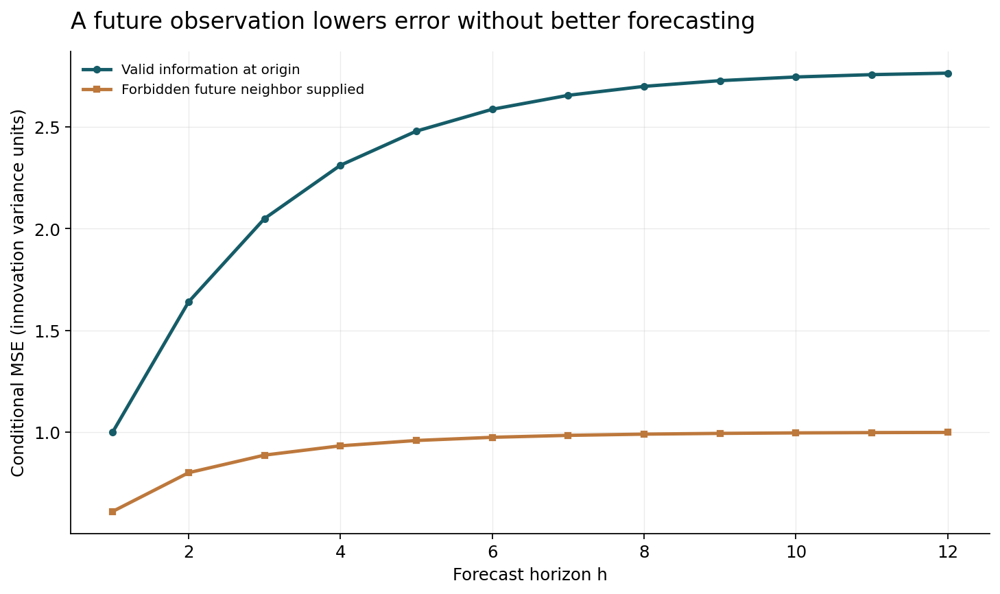
Now provide X_(t+h) itself as an input while still calling the output an h-step forecast. The apparent error can be zero through copying. This extreme control is useful because it exposes the logical issue without any training ambiguity. A subtler version provides X_(t+h+1), a later observation correlated with the target. Conditional Gaussian algebra gives a smaller error than the legitimate forecast even though the model has not become better at predicting from the past. Figure 1 compares the valid error with this future-assisted error. All values are analytic consequences of the declared process, not performance measurements on a real forecasting task.
5. A future proxy can look like a powerful representation
Let V_h denote the legitimate h-step error variance. Since X_(t+h+1)=rho X_(t+h)+epsilon_(t+h+1), conditioning additionally on the future observation reduces the Gaussian conditional variance to V_h sigma squared divided by rho squared V_h plus sigma squared. For rho nonzero this is smaller than V_h. The improvement is entirely explained by information that was unavailable at time t.
This does not mean that every strongly correlated covariate is forbidden. A forecast issued earlier by an independent system may be legitimately available. Its version, issue time, and errors must then be preserved. Replacing it with the subsequently realized value changes the experiment. Similarly, a revised label may be appropriate for measuring final outcomes, while revised inputs may be inappropriate for reconstructing historical decisions. The finite program checks the conditional-variance formula against a covariance-matrix calculation and confirms the rho=0 control, where the future neighbor adds no information. Such controls can reveal leakage in preprocessing before an expensive deep model is trained.
6. Window construction can cross the split
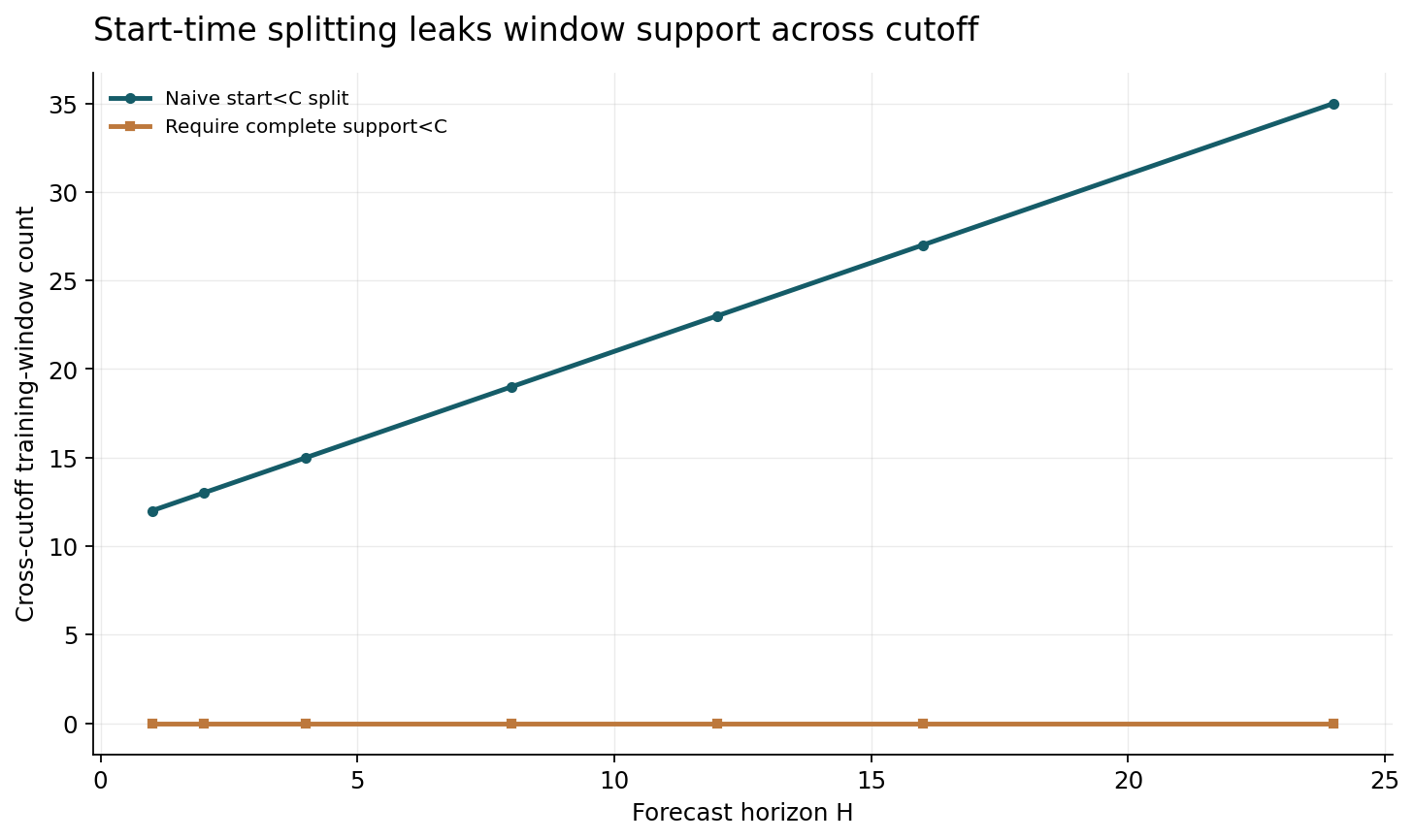
Suppose a training example starts at time s, uses L historical observations, and predicts the following H observations. Its complete support extends from s through s+L+H-1 in discrete time. Assigning examples to training merely because their start time is before a cutoff C can include target observations after C. A test set beginning at C may then share outcomes with training.
The safe condition depends on the intended design. For a strict holdout in which no training target reaches the test period, require s+L+H-1<C. If a rolling-origin procedure legitimately updates the model over time, each update must use only labels already available at that origin. Figure 2 counts training windows that cross the cutoff for several horizons under a deliberately naive start-time split. The construction is an interval audit, not an estimate of accuracy inflation. Shared observations do not automatically imply invalid evaluation in every time-series setting, but they change dependence and the information available. The protocol should explain that dependence rather than treat overlapping windows as independent samples.
7. Normalization can carry future information
A mean or variance estimated from the full series contains information from the evaluation period. Whether this invalidates a claim depends on the task. In a genuinely prospective forecast, a global scaler fitted on future observations is unavailable at deployment. In a transductive task with a known unlabeled batch, the information contract is different and should be stated explicitly. The same numerical operation can therefore be legitimate in one experiment and leakage in another.
Fit transformations inside each training fold or at each rolling origin using the admissible history. Preserve learned scaling parameters and apply them unchanged to the corresponding evaluation segment. Per-instance normalization needs equally careful examination: statistics computed from an input context are available, while statistics computed from the target horizon are not. Missing-value imputation and seasonal decomposition can also use future observations implicitly. A centered moving average, for example, has a different availability requirement from a trailing average. The audit should inspect the actual code path and data dependencies rather than assume that a preprocessing function is harmless because it does not use labels explicitly.
8. Hyperparameter selection has its own clock
Repeatedly evaluating many model variants on a nominal test interval makes that interval part of the selection process. The selected score is then optimistically biased even if every individual prediction used only past inputs. This is a form of evaluation contamination distinct from feature leakage. A final untouched period or a nested temporal validation design is needed to assess the chosen procedure.
The selection object includes more than architecture width and learning rate. Look-back length, forecast horizon, normalization, covariate choice, missing-value rules, checkpoint selection, and random seed selection can all be tuned against future outcomes. Record which interval informed each choice and retain failed trials. If deployment involves periodic retraining, evaluate that entire schedule rather than choosing the best retrospective checkpoint for each horizon. The appropriate unit of comparison is the decision procedure available at the time, including its selection budget. Otherwise a simple baseline with one fixed configuration can be unfairly compared with a neural method selected from an extensive search that repeatedly consulted the test outcomes.
9. Global models introduce cross-series availability
A model trained across many related series can share useful information, but each series may have a different publication delay or observation schedule. An observation from another entity at the same event time may or may not be available when the target entity's forecast is issued. The correct information set is therefore a collection of timestamped records across entities, not just a prefix of one array.
Cross-sectional normalization, embeddings, and aggregate features can quietly use records from later in the operational timeline. Grouped splits also matter when closely related entities share a common hidden process. A model might generalize well to later times for known entities while failing on new entities; those are different tasks. Evaluate temporal and entity generalization separately before combining them. A strong protocol specifies whether entities may appear in both training and evaluation, whether aggregate statistics are recomputed prospectively, and how delayed updates are handled. These details are especially important when a global model's advantage comes from pooling information rather than from a more expressive temporal architecture.
10. Forecast error should be reported by horizon and regime
A single average across horizons can conceal failure at the decision horizon that matters. Likewise, averaging across series can let high-volume or low-variance entities dominate a metric. Scaling choices determine whether errors are comparable, and zero or nearly constant targets can make percentage-based metrics unstable. The metric should be connected to the operational decision rather than selected only because it yields a favorable ranking.
Report horizon-specific errors and relevant uncertainty summaries. For probabilistic forecasts, calibration and sharpness should be evaluated together under the same admissible information. For point forecasts, compare with persistence, seasonal, and appropriately fitted linear baselines. Breakdowns by regime, data availability, and retraining age can reveal whether an apparent overall gain depends on a narrow condition. Confidence intervals should account for temporal dependence and repeated use of overlapping targets. Treating every window as an independent replicate can produce implausibly narrow intervals. The constructed examples do not estimate such intervals; they show why the experimental unit and dependence structure must be defined before uncertainty is calculated.
11. Missingness is sometimes a message
A sensor's absence or a delayed report can carry information about the process being forecast. Masking missing entries at random during training may not reproduce this mechanism. Conversely, filling missing values using observations that arrive later can leak future information. The model should distinguish an absent value, a not-yet-arrived value, a known zero, and an imputed estimate.
At each origin, preserve a mask and an age-since-observation field when appropriate. Evaluate under realistic arrival patterns and outages, not only under independent synthetic masking. If an imputation model is used, fit it within the same temporal boundary as the forecaster and retain its uncertainty. A useful negative control deliberately delays a covariate to see whether performance changes as expected. An unexpectedly unchanged score can indicate that the covariate was unused; an implausibly large improvement from a future-only channel can reveal leakage. Neither outcome alone establishes a causal explanation, but both provide concrete evidence for further investigation of the data path.
12. A prospective replay is stronger than a retrospective table
The most convincing evaluation replays the information state at historical forecast origins. For each origin, load only records available at that time, apply the then-valid preprocessing and model version, generate predictions, and store them before joining final outcomes for scoring. This separates prediction creation from outcome evaluation and makes the provenance of each forecast inspectable.
A replay should include retraining triggers, computation deadlines, and failure handling. If a model cannot finish before a decision deadline, its offline accuracy is not the entire result. If a source feed is delayed, the fallback should be evaluated rather than silently substituting complete retrospective data. Immutable prediction records can prevent accidental recomputation after inspecting outcomes. This does not require a complex production platform for an initial study; a small timestamped experiment ledger can establish the principle. The essential property is that the evidence preserves what the predictor knew, which code and parameters it used, and when the prediction became available.
13. What the constructed checks establish
The accompanying standard-library program derives legitimate autoregressive forecast variances, verifies future-assisted conditional variances through an independent covariance calculation, checks zero-correlation and one-step limits, and enumerates window supports across a cutoff. Its two figures are generated from those declared calculations. No real series, private data, trained weights, or external forecasting service is used.
These checks establish that the examples behave as claimed. They do not prove that a particular published dataset contains leakage or that one architecture is superior. The autoregressive model assumes stationarity, Gaussian innovations for the conditional-variance interpretation, and known parameters. Real datasets may be nonstationary, nonlinear, delayed, or subject to interventions. The interval audit deliberately isolates overlap rather than estimating its effect on error. Those limitations make the controls useful: their expected answers are explicit. A researcher can add them to a pipeline test suite and then design domain-specific checks for the actual data-generating and data-arrival processes.
14. A timestamp audit can be tested without a model
Before fitting any predictor, construct a lineage table for each feature. Record the latest source availability time that could influence it. A trailing average inherits the latest availability time of its included observations; a learned scaler inherits the latest time used in fitting; an imputed value inherits both its conditioning records and the imputer's training boundary. The final feature is admissible only when these dependencies precede the forecast origin under the declared contract.
This audit can be implemented on a small synthetic timeline with deliberately delayed records. Insert a future-only sentinel feature and require the pipeline to reject it. Add a calendar covariate known in advance and require the pipeline to accept it. Add a revised historical observation whose later version was unavailable at the origin and verify that the original vintage is selected. These positive and negative controls test the information boundary more directly than checking whether model accuracy seems plausible.
A prediction ledger should also retain the target horizon and outcome definition. If outcomes are revised, scoring against the first release and against the final release answers different questions. Both can be reported, but the choice must not change after inspecting which one favors a model. This is especially relevant when the practical decision concerns a value as initially published. The review does not implement a production lineage system; it specifies concrete tests that can make the time contract executable before architectural comparisons begin.
15. The benchmark is a simulation of a decision
A forecasting benchmark should simulate a decision made with incomplete information, not merely reward reconstruction of a completed historical table. The distinction places timestamp provenance, preprocessing, selection, and execution deadlines alongside model design. An architecture comparison that ignores those components can yield a precise number for an ill-defined task.
The analytical future-proxy example and the window-support audit demonstrate two separate ways to violate the intended boundary. Both can make a model appear stronger without improving its ability to forecast from the available past. Future work should publish availability-aware datasets, versioned prediction ledgers, and evaluation code that makes forbidden dependencies fail visibly. Such practices would allow gains from representation learning to be interpreted with greater confidence. Until then, the most important question about a forecasting score is often not how many parameters produced it, but whether the information used to produce it existed when the forecast was supposed to be made.
Core equations and definitions
(1) Stationary Gaussian autoregression with independent innovations of variance sigma squared.
(2) Valid conditional mean at origin t with known rho.
(3) Valid h-step forecast error variance.
(4) Conditional variance when the forbidden future observation X_(t+h+1) is supplied.
(5) A strict training window with look-back L, horizon H and start s must finish before cutoff C.
Constructed analytical figures
Comparison and reporting contract
| Diagnostic | What it establishes | What remains unproved |
|---|---|---|
| Low test error | Score under supplied information | Prospective validity |
| Past event timestamp | When event occurred | When value was available |
| Random window split | A partition of rows | Independent temporal holdout |
| Known calendar covariate | Future event with available value | Permission to use future realized measurements |
Evaluation protocol
- Record event and availability timestamps.
- Fit all transformations within the allowed history.
- Audit complete window support across cutoffs.
- Separate validation selection from final evaluation.
- Replay model versions and prediction deadlines before joining outcomes.
Limitations
- No real forecast dataset or neural model is used.
- Conditional variance assumes a Gaussian stationary process with known parameters.
- Window overlap counts do not quantify accuracy inflation.
- No cited benchmark is alleged to contain leakage.
Open research questions
- How can feature lineage make availability constraints executable?
- Which evaluation designs best represent delayed and revised feeds?
- How should uncertainty account for overlapping targets and retraining?
Evidence and its boundaries
- Time representation is a modeling choice separate from architecture.
- [1] — Scope-level source statement only; no independent reproduction, priority ranking or theorem-proof audit. Inspected: Primary author abstract and bibliographic record.
- Known future covariates are distinguished from historically observed inputs.
- [2] — Scope-level source statement only; no independent reproduction, priority ranking or theorem-proof audit. Inspected: Primary author abstract and bibliographic record.
- Efficient attention and multi-step decoding address long-horizon forecasting.
- [3] — Scope-level source statement only; no independent reproduction, priority ranking or theorem-proof audit. Inspected: Primary author abstract and bibliographic record.
- Linear baselines challenge studied transformer forecasting comparisons.
- [4] — Scope-level source statement only; no independent reproduction, priority ranking or theorem-proof audit. Inspected: Primary author abstract and bibliographic record.
- Patching and channel independence are studied for transformer forecasting.
- [5] — Scope-level source statement only; no independent reproduction, priority ranking or theorem-proof audit. Inspected: Primary author abstract and bibliographic record.
- A recurrent probabilistic forecaster learns across related time series.
- [6] — Scope-level source statement only; no independent reproduction, priority ranking or theorem-proof audit. Inspected: Primary author abstract and bibliographic record.
References
- Time2Vec: Learning a Vector Representation of Time
Seyed Mehran Kazemi, Rishab Goel, Sepehr Eghbali, Janahan Ramanan, Jaspreet Sahota, Sanjay Thakur, Stella Wu, Cathal Smyth, Pascal Poupart, Marcus Brubaker. arXiv author manuscript (2019). https://arxiv.org/abs/1907.05321Source scope
Primary author record title, complete author list, submission history and abstract inspected through web tools on 2026-10-28. Full proof and benchmark execution not independently checked.
- Temporal Fusion Transformers for Interpretable Multi-horizon Time Series Forecasting
Bryan Lim, Sercan O. Arik, Nicolas Loeff, Tomas Pfister. arXiv author manuscript (2019). https://arxiv.org/abs/1912.09363Source scope
Primary author record title, complete author list, submission history and abstract inspected through web tools on 2026-10-28. Full proof and benchmark execution not independently checked.
- Informer: Beyond Efficient Transformer for Long Sequence Time-Series Forecasting
Haoyi Zhou, Shanghang Zhang, Jieqi Peng, Shuai Zhang, Jianxin Li, Hui Xiong, Wancai Zhang. arXiv author manuscript (2020). https://arxiv.org/abs/2012.07436Source scope
Primary author record title, complete author list, submission history and abstract inspected through web tools on 2026-10-28. Full proof and benchmark execution not independently checked.
- Are Transformers Effective for Time Series Forecasting?
Ailing Zeng, Muxi Chen, Lei Zhang, Qiang Xu. arXiv author manuscript (2022). https://arxiv.org/abs/2205.13504Source scope
Primary author record title, complete author list, submission history and abstract inspected through web tools on 2026-10-28. Full proof and benchmark execution not independently checked.
- A Time Series is Worth 64 Words: Long-term Forecasting with Transformers
Yuqi Nie, Nam H. Nguyen, Phanwadee Sinthong, Jayant Kalagnanam. arXiv author manuscript (2022). https://arxiv.org/abs/2211.14730Source scope
Primary author record title, complete author list, submission history and abstract inspected through web tools on 2026-10-28. Full proof and benchmark execution not independently checked.
- DeepAR: Probabilistic Forecasting with Autoregressive Recurrent Networks
David Salinas, Valentin Flunkert, Jan Gasthaus. arXiv author manuscript (2017). https://arxiv.org/abs/1704.04110Source scope
Primary author record title, complete author list, submission history and abstract inspected through web tools on 2026-10-28. Full proof and benchmark execution not independently checked.