

Abstract
Graph neural networks propagate information through neighborhood aggregation, but aggregator distinguishability, mixing through repeated propagation, and graph-splitting procedures jointly determine the results. This article compares GCN, GIN, and neighborhood sampling ideas, distinguishes oversmoothing from oversquashing, and calculates changes in variance after repeated averaging on a six-node path graph. The accompanying figure involves no trained parameters and does not represent accuracy on real graph tasks.[1] Semi-Supervised Classification with Graph Convolutional[2] How Powerful are Graph Neural Networks?[3] Inductive Representation Learning on Large Graphs
English abstract
Message-passing graph networks are analyzed through normalized aggregation, permutation behavior and multiset distinguishability. A six-node path calculation illustrates smoothing for one declared propagation operator. It is not a universal oversmoothing theorem or model benchmark. Graph-level and temporal splits, feature provenance and inductive access rules are required for credible evaluation.
1. Neighborhood aggregation should respect node relabeling
Node numbering should generally not change the meaning of a graph, so node representations should transform correspondingly under relabeling, while graph-level outputs should remain invariant. Normalized adjacency propagation and shared parameters can satisfy this structural requirement, but IDs or split information in the features may still introduce leakage. Self-loops and degree normalization in GCN change the propagation scale. Whether the graph is directed or weighted, along with the self-loop rules, should be recorded; an implementation cannot be adequately described merely as “using GCN.”[1] Semi-Supervised Classification with Graph Convolutional
2. Whether an aggregator can distinguish multisets is crucial
Mean, sum, and maximum aggregation may produce identical results for different neighborhoods; for example, mean aggregation conflates different multisets that have the same mean. GIN investigated the relationship between message-passing networks and graph distinguishability. Its conclusions depend on function classes and assumptions and should not be interpreted as meaning that any trained GIN can distinguish all graphs. Structural indistinguishability should also be separated from a failure to learn during optimization: increasing the number of training epochs cannot repair the information loss inherent in a particular fixed aggregator.[2] How Powerful are Graph Neural Networks?
3. Repeated mixing may cause representations to converge
Under fixed linear propagation, neighborhood averaging gradually mixes node information; its long-term behavior can be analyzed under specific connectivity and spectral conditions. Actual networks include nonlinearities, residual connections, normalization, and trained weights, so a variance curve from simple averaging cannot be treated as a theorem for all GNNs. This article applies row normalization to a six-node path after adding self-loops and directly iterates a fixed input vector to illustrate convergence under this operator; classification quality was not measured.[1] Semi-Supervised Classification with Graph Convolutional
4. Oversmoothing and oversquashing are different bottlenecks
Representation convergence emphasizes the difficulty of distinguishing different nodes; oversquashing emphasizes the compression of large amounts of distant information through limited width or a small number of edges. A graph task may require only local information, or it may require long-range relationships across the graph. Increasing depth expands the receptive field while also changing optimization and information mixing. Tests should be constructed to separate local and long-range requirements, with structure, width, residual connections, and sampling ablated separately. Poor performance at greater depth should not simply be attributed to a single cause.[2] How Powerful are Graph Neural Networks?[3] Inductive Representation Learning on Large Graphs
5. Inductive and transductive evaluation differ in accessible information
A transductive setting may allow the graph structure of unlabeled test nodes to be visible during training, whereas an inductive setting requires generalization to new nodes or new graphs. GraphSAGE investigated inductive representations through sampling and aggregation, but an implementation must specify which edges and features are accessible during training. If edges from later times or features derived from target labels enter training, leakage may inflate scores. Random node splits do not automatically represent generalization to new graphs, future relationships, or new institutions.[3] Inductive Representation Learning on Large Graphs
6. Graph experiments require both structural and systems verification
Record the graph version, deduplication, self-loops, edge directions, feature provenance, and splits, and isolate related samples by graph family or time. Report results across multiple seeds, class-stratified results, and gains over simple feature-based baselines. Sampling on large graphs also requires measuring coverage, communication, and memory, and distinguishing sampling approximations from full-neighborhood results. This article only computes a propagation operator; it does not claim to have trained a new graph model or achieved benchmark results.[1] Semi-Supervised Classification with Graph Convolutional[2] How Powerful are Graph Neural Networks?[3] Inductive Representation Learning on Large Graphs
Core equations and derivations
(1) Illustration of GCN-style symmetric normalization; definitions of direction, weights, self-loops, and degrees should match the implementation.
LaTeX
H^{\prime}=\sigma(\tilde D^{-1/2}\tilde A\tilde D^{-1/2}HW),\quad\tilde A=A+I(2) GIN-style sum aggregation; distinguishability analysis is subject to function-class conditions, not a universal guarantee for actual training.
LaTeX
h_v^{\prime}=\operatorname{MLP}\left((1+\epsilon)h_v+\sum_{u\in N(v)}h_u\right)(3) The figure in this article uses a six-node path and this row-stochastic operator, which differs from the symmetric normalization above; the distinction is made explicit to avoid confusion.
LaTeX
x^{(k)}=P^kx^{(0)},\quad P=D^{-1}(A+I)Method and evidence workflow
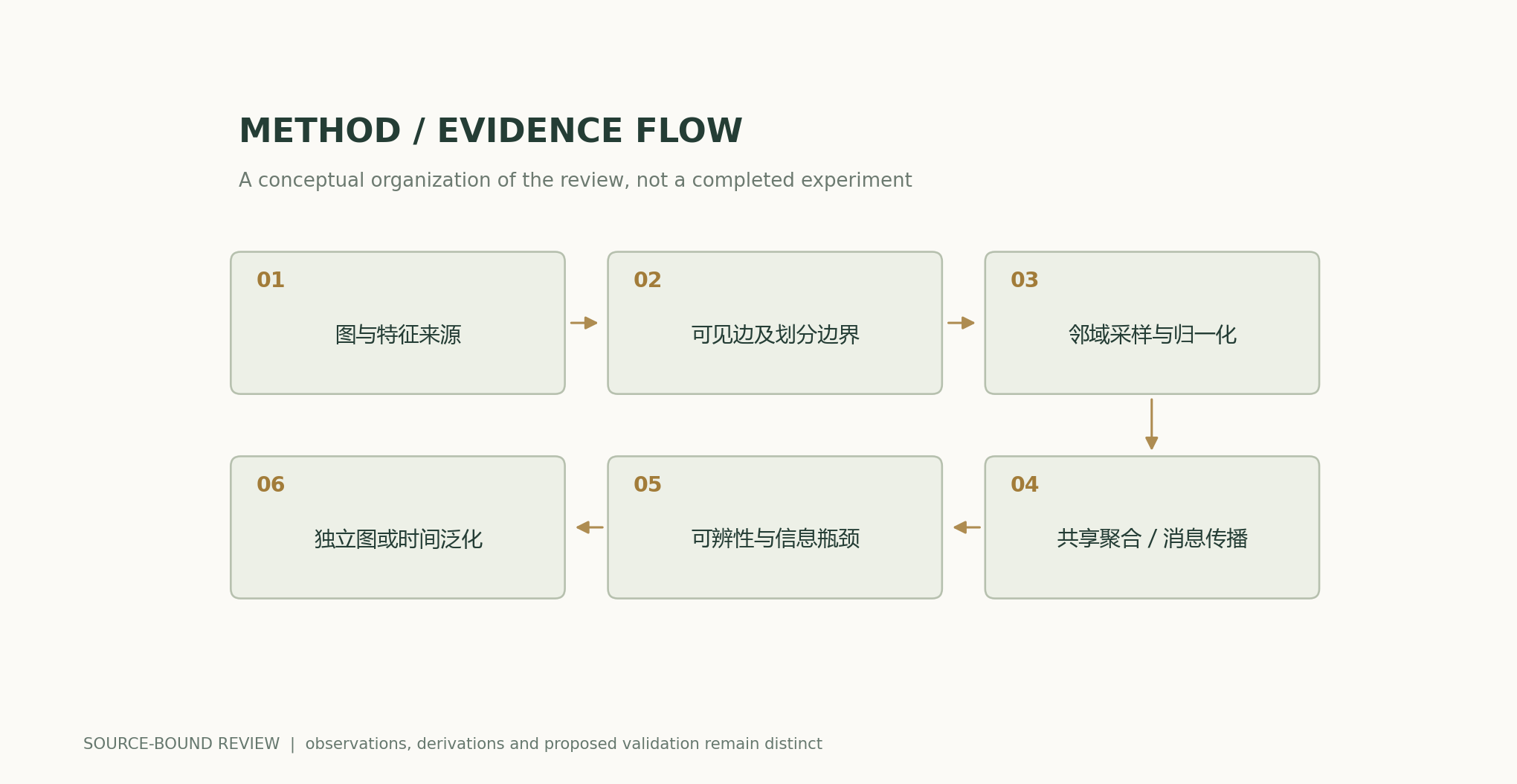
Analytical figures and numerical examples
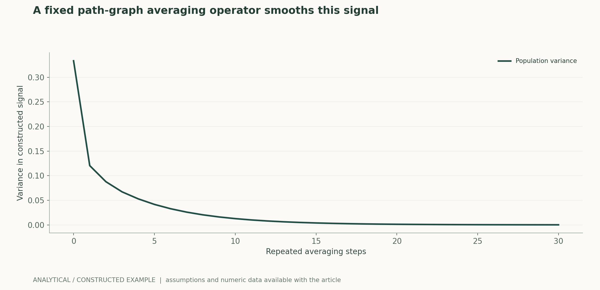
Recomputable worked example
The initial population variance is 0.333333, and it is approximately 0.012679 after 10 propagation steps with this operator. Nonlinearities, residual connections, and trained weights change the behavior; actual classification quality cannot be inferred from this calculation.
Method comparison
| Method or judgment | Controlled variables and measurements | Failure conditions and interpretation |
|---|---|---|
| Normalized propagation | Record direction, self-loop, and degree rules | Architectures with the same name may use different operators |
| Mean and sum | Construct controlled comparisons of multiset distinguishability | More training does not resolve structural indistinguishability |
| Deep propagation | Measure convergence and long-range information requirements separately | Oversmoothing and oversquashing must not be conflated |
| Graph splitting | Specify transductive/inductive access and temporal visibility | Random node splits may introduce leakage |
Verification and experimental plan
- Freeze the versions of the graph, feature provenance, edge directions, self-loops, and deduplication.
- Specify transductive or inductive access boundaries, and split by time or graph family.
- Check aggregation outputs through node relabeling and hand calculations on small graphs.
- Compare simple feature-based baselines, different aggregators, depths, and residual connections to isolate structural factors.
- Use local and long-range tasks and multiple seeds; report stratified quality and graphs on which the method fails.
- For large graphs, jointly measure sampling coverage, peak memory, and time, retaining a full-neighborhood reference.
Scope and limitations
- The path-graph propagation has no trained weights.
- Declining variance is not a theorem for all GNNs.
- An upper bound on expressivity does not guarantee successful optimization.
- Transductive scores cannot automatically be extrapolated to inductive tasks.
Mapping primary sources to claims
- Semi-Supervised Classification with Graph Convolutional Networks, · 2016-09-09Abstract; 原文方法、理论和实验章节见作者原始论文链接
- How Powerful are Graph Neural Networks?, , , · 2018-10-01Abstract; 原文方法、理论和实验章节见作者原始论文链接
- Inductive Representation Learning on Large Graphs, , · 2017-06-07Abstract; 原文方法、理论和实验章节见作者原始论文链接
Citation and article export
BibTeXRISCSL JSONTXTArticle JSON
Author, version, and sources
An AI-assisted research review; Codex (AI) wrote the article and performed analytical derivations based on the listed primary literature. This site has no record of independent peer review or original model experiments for this article.
Reader performance revision: previously read pages are also reused when a recent HEAD request returns 200 and the ETag matches. The main text, equations, sources, and scientific figure data retain the content of the previous version.
The conceptual cover is separate from the scientific diagrams; scientific figures are computed from publicly available equations and explicitly stated assumptions, and all results from original papers are attributed.
Author, version, and correction history · /guides/graph-neural-networks/v1/
Cover and scientific figure sources · Data, sources, and assumptions · Publication and version history
Source revision: 6251a250b27bb8b449f59b392f81abd355383770