
Deep Learning: Sequence Models / DEEP LEARNING III
Learning Inside the Context: Bayesian Ambiguity and Algorithmic Imitation
Successful in-context prediction does not uniquely identify the algorithm implemented by a sequence model.
English original. Translations of this new review are not yet available.

Abstract
Successful in-context prediction does not uniquely identify the algorithm implemented by a sequence model. This review separates behavioral equivalence, Bayesian interpretation, activation-level computation and causal mechanism. An exact two-hypothesis construction shows how different priors remain consequential after ambiguous demonstrations, while a ridge-regression control shows when iterative and closed-form learners can agree. The analysis motivates interventions that distinguish mechanisms instead of treating one matched output as proof of an internal learning rule.
In this paper
- 1. A prediction can have several explanations
- 2. What the six source records establish
- 3. Define the task before defining the learner
- 4. A two-hypothesis ambiguity construction
- 5. Repetition is not independent evidence by default
- 6. A discriminating observation changes the posterior
- 7. Behavioral agreement does not identify a mechanism
- 8. A scalar regression control
- 9. Matching an update rule requires more than a curve
- 10. Order can reveal the inferred statistical model
- 11. Demonstrations carry format and semantics
- 12. Mechanistic probes need causal discipline
- 13. Generalization tests should challenge the explanation
- 14. What the executable analysis checks
- 15. A reporting hierarchy
- 16. Research directions and limitations
1. A prediction can have several explanations
A language model can change its answer after seeing examples in a prompt even though its weights remain fixed. This behavior is often described as learning in context. The description is useful, but it leaves open what computation produced the adaptation. The model might infer a latent task, imitate a familiar pattern, implement an approximate update rule, retrieve a memorized template or combine several strategies.
The scientific problem is therefore one of identification. Many internal procedures can agree on a finite set of prompts. Observing agreement with a Bayesian predictor or a gradient-descent learner does not by itself establish that the model implements that mechanism. This review develops two exact controls: a finite Bayesian task mixture with ambiguous examples, and a scalar regression problem where closed-form and iterative learners can coincide at selected points. These constructions clarify which interventions can distinguish hypotheses. They are not experiments on a pretrained language model. Their purpose is to improve the logic connecting behavioral measurements to claims about in-context learning, while acknowledging that multiple explanations may remain observationally equivalent under the available tests.
2. What the six source records establish
Xie and colleagues analyze implicit Bayesian inference in a specified latent-concept pretraining setting. Garg and colleagues study in-context learning of simple function classes. Akyurek and colleagues investigate learning algorithms using linear models, while von Oswald and colleagues examine connections to gradient descent in controlled Transformer settings. These are valuable results with explicit model and task assumptions.
Min and colleagues study what demonstrations contribute on selected language tasks, including interventions on labels. Olsson and colleagues investigate induction heads and their relationship to in-context behavior. These records motivate both algorithmic and mechanistic hypotheses, but they do not make every observed context adaptation an instance of one universal procedure. Our source inspection covers the original abstracts and bibliographic metadata. Complete proofs, circuits and training runs are not independently replicated here. The authored examples below use elementary probability and optimization to expose ambiguity in interpreting finite behavioral tests. They show why a controlled construction can demonstrate possibility, while an empirical mechanism claim requires additional evidence about the trained model and the domain on which the claim is intended to hold.
3. Define the task before defining the learner
An in-context example is meaningful only relative to a task distribution. In a regression setting, examples may be pairs of numerical inputs and outputs generated by a hidden function. In a language classification setting, labels, formatting and semantic priors can all influence the answer. A demonstration may identify the label vocabulary without teaching the input-output relation from scratch.
The evaluation should specify which aspects of the task are new. Are the labels remapped? Are inputs drawn from a new distribution? Is the underlying function family familiar from training? Does the query require extrapolation outside the demonstration range? These choices alter what success establishes. A model that follows a novel label mapping has demonstrated a different capability from one that recognizes familiar sentiment labels. Likewise, predicting within a trained function family differs from discovering an arbitrary new rule. Treating both as one learning score hides the inductive assumptions. A rigorous study describes the latent task, the prompt-generation process and the query distribution, then asks which candidate algorithms make different predictions under controlled changes to those elements.
4. A two-hypothesis ambiguity construction
Consider two possible functions on binary inputs. Hypothesis H0 returns the input unchanged; hypothesis H1 returns zero for both inputs. Every demonstration with input zero and output zero is equally compatible with both hypotheses. No matter how many exact duplicates of that example appear, they provide no likelihood ratio favoring one hypothesis in the noiseless construction.
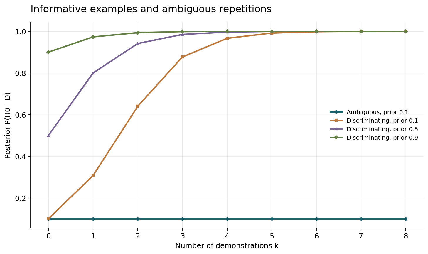
Let the prior probability of H0 be pi. After any number of these ambiguous demonstrations, the posterior remains pi. For a query at input one, the posterior probability that the latent noiseless function returns one is therefore pi. This latent-function probability must be distinguished from the predictive probability of a future noisy observed label. Two Bayesian learners with different priors disagree even though they observe the same demonstrations and both update correctly. Figure one displays the posterior probability of H0 as ambiguous examples accumulate, alongside the effect of discriminating examples under a declared noisy observation model. The construction does not claim that a language model literally represents these two hypotheses. It shows that a prompt's apparent amount of evidence is not the same as its ability to distinguish tasks, and that prior assumptions remain consequential when the demonstrations are uninformative.
5. Repetition is not independent evidence by default
If repeated demonstrations are exact copies of one observation, treating them as independent noisy samples can overstate their information. A probabilistic model must specify whether repetitions represent new draws, duplicated records or deliberate emphasis. These interpretations produce different posteriors even when the visible prompt text is similar.
In the noiseless ambiguity example, repeated zero-input pairs remain uninformative under all reasonable duplicate handling because both hypotheses predict them identically. Under noisy labels, repeated observations at a discriminating input can accumulate evidence only if the independence assumption is justified. A model that interprets repetition as rhetorical emphasis may behave differently from a statistical learner. This is not automatically irrational; it may reflect the distribution on which the model was trained. An evaluation seeking a Bayesian interpretation should therefore test duplication separately from independent resampling. It should also vary formatting and order without changing the underlying statistical information. These controls help identify whether the model responds to evidence quantity, token frequency, recency or a learned discourse convention.
6. A discriminating observation changes the posterior
Introduce independent label noise with error probability epsilon below one half. At input one, observing output one has likelihood one minus epsilon under H0 and epsilon under H1. After k independent such observations, posterior odds equal prior odds multiplied by the likelihood ratio raised to k.
The formula makes the assumptions inspectable. A larger k increases confidence only because the observations are modeled as independent and the noise rate is known. If the noise rate is misspecified, the posterior can become overconfident. If observations are duplicated, multiplying the likelihood repeatedly is unjustified. Figure one uses epsilon equal to one fifth and several priors, so the posterior moves at different rates from different starting beliefs. The finite program verifies the odds update against direct Bayes normalization. The point is not that one prior is correct universally. It is that a claim about Bayesian behavior requires identifying both the likelihood model and the prior, and showing that the model's responses track interventions that separate them.
At input one, the latent function equals one exactly when H0 holds, so its posterior probability is P(H0 given D). A future observed label has an additional independent error: its predictive probability of one is epsilon plus (one minus twice epsilon) times P(H0 given D). With epsilon equal to 0.2, this is 0.2 plus 0.6 times the plotted posterior. Figure one deliberately plots the hypothesis posterior, not the noisy-label prediction; even a posterior approaching one leaves the latter approaching 0.8.
7. Behavioral agreement does not identify a mechanism
Suppose a neural model matches the Bayesian predictive probability on a finite set of prompts. A lookup table over those prompts would match as well. A simpler heuristic might also agree because the test set does not include cases where its predictions diverge. The issue is not that Bayesian explanations are useless, but that agreement is evidence of compatibility rather than uniqueness.
Mechanism identification needs interventions chosen to distinguish alternatives. Vary the prior information while holding examples fixed; change the noise process; duplicate observations without adding information; query outside the demonstration support. A candidate learner should make predictions before the intervention results are inspected. If several mechanisms remain equivalent, report that equivalence rather than selecting the most appealing story. Internal measurements can add evidence, but they too need causal controls. A representation correlated with a posterior statistic does not prove that the statistic drives the output. The strongest account combines behavioral predictions, internal state measurements and interventions that alter the proposed computation while preserving unrelated capabilities as much as possible.
8. A scalar regression control
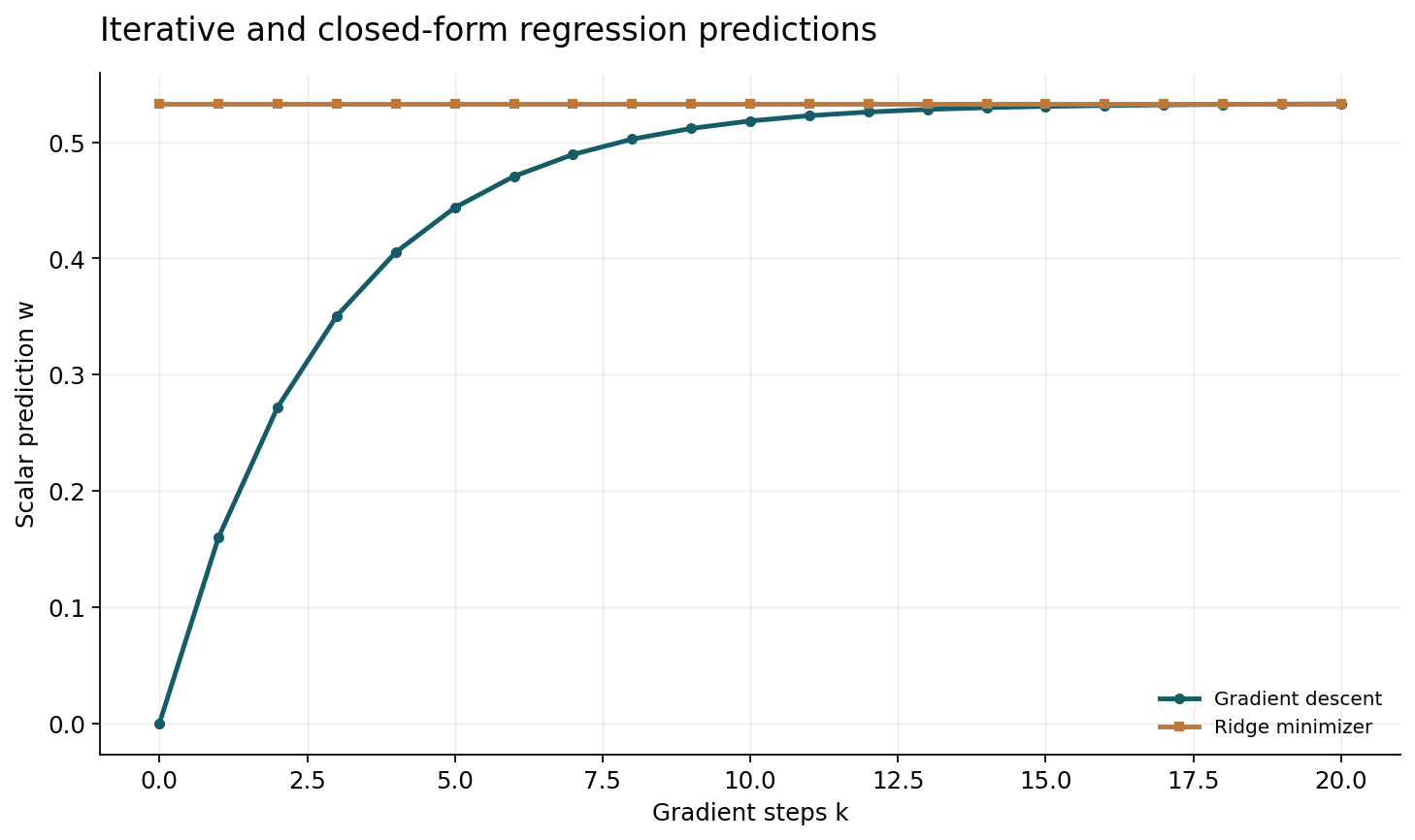
Consider observations with input x equal to one and average target ybar. A regularized squared-error objective has minimizer ybar divided by one plus lambda. Starting from zero, gradient descent with step eta follows a geometric recurrence whose solution is ybar times one minus q to the k, divided by one plus lambda, where q equals one minus eta times one plus lambda.
An iterative learner and the closed-form ridge solution can be arbitrarily close after enough steps. At a particular step size, they can even agree after one update in this scalar setting. Observing one final prediction therefore cannot identify whether the model used an iterative computation, a direct formula or another equivalent map. Figure two plots the iterative estimate against the fixed minimizer under a declared stable step. This is an optimization control, not a claim that a Transformer performs exactly that recurrence. Its value is that the possible equivalence is explicit. A discriminating test must vary the data geometry, regularization or number of effective updates rather than relying on a single easy scalar instance.
9. Matching an update rule requires more than a curve
A model whose outputs resemble several steps of gradient descent on one task family may still implement a different procedure that approximates the same solution. To strengthen the update-rule hypothesis, test conditions where candidate algorithms differ: anisotropic features, rescaled inputs, correlated examples, nonzero initialization or altered regularization.
The hypothesis should specify what counts as an iteration and where the state of the implied learner resides. A layer may correspond only approximately to an update, and the correspondence may depend on the prompt length. If a model has learned a direct estimator, forcing an iterative interpretation can introduce unnecessary hidden assumptions. Conversely, an approximate iterative mechanism may be useful even if it does not exactly match textbook gradient descent. The report should distinguish exact construction, fitted behavioral surrogate and causal mechanism. These are different evidence levels. A concise mathematical fit is an explanatory tool, not proof that the trained network follows the fitted algorithm internally. Testing out-of-family cases helps determine whether the fit captures a robust computation or only a narrow coincidence.
10. Order can reveal the inferred statistical model
For an exchangeable Bayesian dataset with conditionally independent examples, permuting the examples leaves the posterior unchanged. An online optimizer with a finite number of order-dependent updates may not have that property. A sequence model can also exhibit recency or formatting effects unrelated to either idealized learner.
Order interventions are therefore useful, but their interpretation must respect the task. In a temporally evolving process, order carries real information and permutation should change the answer. In a static regression dataset, it may be irrelevant. A benchmark should explicitly distinguish these regimes. When order is semantically irrelevant, measure the distribution of predictions over permutations and compare it with candidate algorithms. When order is meaningful, include controlled changes that preserve or reverse the temporal relation. An observed order effect does not by itself prove gradient descent; many sequence heuristics can produce it. It narrows the set of compatible explanations only when the competing models make specific, differing predictions under the same prompt-generation assumptions.
11. Demonstrations carry format and semantics
Language examples can communicate output format, label meanings, domain vocabulary and the intended level of detail. Removing or randomizing labels may leave some of these signals intact. Thus a small performance change after label perturbation need not mean that the model learned an arbitrary task without supervision, nor that demonstrations never matter.
A factorial design separates label mapping, input distribution, formatting and example-answer correspondence. It can use novel symbols to reduce semantic label priors, but those symbols introduce their own tokenization and frequency effects. It can paraphrase instructions while retaining the statistical task, but paraphrases may vary in clarity. These limitations should be documented rather than treated as reasons to avoid controlled tests. The goal is to identify which information in the prompt drives adaptation. For a familiar task, a model may mainly infer what is being requested. For a novel function family, it may need to infer a new mapping. Both behaviors are useful, but they support different conclusions about the scope of in-context learning.
12. Mechanistic probes need causal discipline
An internal activation may correlate with a task parameter, a posterior probability or an intermediate regression estimate. Such a probe can reveal useful organization, but a flexible probe may extract a statistic that the model never uses. The distinction between decodability and causal role is central.
Interventions should target the proposed representation and test predicted changes in output, while measuring collateral damage. Replacing an activation with an out-of-distribution vector can break the network for reasons unrelated to the hypothesized mechanism. Patching between carefully matched prompts can reduce that problem, but matching itself requires assumptions. A circuit-level account should state its scope: which models, layers, tasks and prompt lengths were tested. It should also retain examples where the proposed mechanism fails. The present review performs no activation analysis. It supplies a conceptual standard for interpreting one: a successful probe is evidence about recoverability, a successful intervention adds evidence about causal contribution, and neither automatically establishes that the mechanism is universal across in-context tasks.
13. Generalization tests should challenge the explanation
If a model is claimed to infer a Bayesian task posterior, test changes in prior frequencies and observation noise. If it is claimed to implement a regression algorithm, test feature covariance, scaling and regularization. If it is claimed to copy induction patterns, test controlled breaks in the relevant repetition structure. The evaluation should be tailored to the explanation rather than merely adding more examples from the same easy distribution.
Hold out entire task families or parameter regimes where possible. Report failures alongside successes and distinguish interpolation in the task distribution from extrapolation beyond it. Prompt selection must not be tuned on the final test cases. Multiple random seeds for synthetic task generation help quantify variability, but they do not replace diversity of task structure. A model can perform well on many samples from a narrow generator while failing on a small structural change. The exact constructions in this article make that point: ambiguous and discriminating examples can have the same length, yet differ radically in what they establish about the latent task.
14. What the executable analysis checks
The companion program enumerates the two hypotheses, computes likelihoods for ambiguous and discriminating observations, and verifies posterior normalization. It confirms that repeated ambiguous examples leave the posterior unchanged. It compares direct normalization with the odds formula under independent noisy discriminating observations and checks equal-prior symmetry. It separately verifies the future noisy-label mixture against the affine posterior formula.
For the regression control, it evaluates the iterative recurrence and the closed-form expression at several step counts, verifies convergence under the chosen stable step, and checks the one-step special case when the step equals the reciprocal curvature. The figures are generated from these exact computations. Passing the checks establishes arithmetic consistency and the claimed finite equivalences. It does not establish that any neural model realizes the Bayesian or regression procedure. No weights are trained, no benchmark scores are produced, and no source experiment is replicated. This separation is deliberate: a reproducible counterexample can strengthen the logic of an evaluation without being misrepresented as an empirical discovery about a deployed language model.
15. A reporting hierarchy
A useful report distinguishes four statements. A model can represent a learning algorithm; a trained model behaves similarly on a test set; an internal computation correlates with that algorithm; and a causal intervention supports that computation's role. Each statement requires different evidence, and later statements do not follow automatically from earlier ones.
The hierarchy prevents two opposite errors. One is dismissing a constructive result because it does not prove what every trained model does. The other is treating a constructive possibility as an empirical explanation of a particular model. Both obscure real progress. A precise study can establish a limited but valuable result, such as behavioral equivalence on a controlled function family, while leaving the broader mechanism question open. The finite controls here show why that restraint matters. Prior ambiguity and algorithmic equivalence are not rhetorical objections; they can be written as explicit probabilities and recurrences. A discriminating experiment should therefore be part of the explanation from the beginning, not added only after a preferred story has been chosen.
16. Research directions and limitations
Future work can improve identification by combining task-distribution interventions with internal causal tests and by publishing predictions from competing mechanisms before collecting outcomes. It can also study when a model switches strategies as prompt length, noise or semantic familiarity changes. A single universal account may be less realistic than a mixture of computations selected by context.
The present review remains a selective synthesis with two elementary constructions. It does not adjudicate among all theories of in-context learning, and it does not claim novelty for the basic Bayesian or optimization formulas. Its contribution is an explicit connection between those formulas and the logic of experimental inference. The central caution is constructive: an explanation becomes stronger when it identifies the observations that could distinguish it from alternatives. Successful prediction is the beginning of that inquiry, not its end. A credible account of learning inside the context must state what was learned, which assumptions made it identifiable, and how the proposed computation was tested beyond the cases where many different procedures would have produced the same answer.
Core equations and definitions
(1) Two-hypothesis Bayes normalization.
(2) Independent discriminating observations under label error epsilon.
(3) Scalar ridge objective with unit inputs.
(4) Gradient descent from zero under the stated scalar quadratic.
(5) Predictive probability of a future independently corrupted label, distinct from the latent-function posterior plotted in Figure one.
Constructed analytical figures
Comparison and reporting contract
| Object | What it establishes | What it does not establish |
|---|---|---|
| Constructive representation | An architecture can implement a learner | A trained model uses it |
| Behavioral agreement | Predictions match on tested inputs | The internal mechanism is unique |
| Probe decoding | A statistic is recoverable | It causally controls the output |
Evaluation protocol
- Specify latent tasks, priors, noise and query distribution.
- Separate duplicated records from independent examples.
- Choose interventions where candidate learners disagree.
- Distinguish behavioral fit, decodability and causal mechanism.
Limitations
- No neural model is trained or probed.
- The task mixture has only two hypotheses.
- The regression control is scalar and does not model a complete Transformer.
Open research questions
- When do models switch among different in-context strategies?
- Which interventions identify priors separately from likelihood assumptions?
- How can causal circuit evidence generalize across task families?
Evidence and its boundaries
- Analyzes Bayesian inference in a specified latent-concept setting.
- [1] — Original arXiv bibliographic record and abstract inspected on 2026-10-28; full proof and source experiments not independently audited. Inspected: Primary arXiv abstract and bibliographic record.
- Studies in-context learning of simple function classes.
- [2] — Original arXiv bibliographic record and abstract inspected on 2026-10-28; full proof and source experiments not independently audited. Inspected: Primary arXiv abstract and bibliographic record.
- Investigates learning algorithms using linear-model tasks.
- [3] — Original arXiv bibliographic record and abstract inspected on 2026-10-28; full proof and source experiments not independently audited. Inspected: Primary arXiv abstract and bibliographic record.
- Connects controlled Transformer computations to gradient descent.
- [4] — Original arXiv bibliographic record and abstract inspected on 2026-10-28; full proof and source experiments not independently audited. Inspected: Primary arXiv abstract and bibliographic record.
- Studies the informational role of demonstrations and label interventions.
- [5] — Original arXiv bibliographic record and abstract inspected on 2026-10-28; full proof and source experiments not independently audited. Inspected: Primary arXiv abstract and bibliographic record.
- Investigates induction heads and in-context behavior.
- [6] — Original arXiv bibliographic record and abstract inspected on 2026-10-28; full proof and source experiments not independently audited. Inspected: Primary arXiv abstract and bibliographic record.
References
- An Explanation of In-context Learning as Implicit Bayesian Inference
Sang Michael Xie, Aditi Raghunathan, Percy Liang, Tengyu Ma. arXiv primary author manuscript (2021). https://arxiv.org/abs/2111.02080Source scope
Original arXiv bibliographic record and abstract inspected on 2026-10-28; full proof and source experiments not independently audited.
- What Can Transformers Learn In-Context? A Case Study of Simple Function Classes
Shivam Garg, Dimitris Tsipras, Percy Liang, Gregory Valiant. arXiv primary author manuscript (2022). https://arxiv.org/abs/2208.01066Source scope
Original arXiv bibliographic record and abstract inspected on 2026-10-28; full proof and source experiments not independently audited.
- What learning algorithm is in-context learning? Investigations with linear models
Ekin Akyürek, Dale Schuurmans, Jacob Andreas, Tengyu Ma, Denny Zhou. arXiv primary author manuscript (2022). https://arxiv.org/abs/2211.15661Source scope
Original arXiv bibliographic record and abstract inspected on 2026-10-28; full proof and source experiments not independently audited.
- Transformers learn in-context by gradient descent
Johannes von Oswald, Eyvind Niklasson, Ettore Randazzo, João Sacramento, Alexander Mordvintsev, Andrey Zhmoginov, Max Vladymyrov. arXiv primary author manuscript (2022). https://arxiv.org/abs/2212.07677Source scope
Original arXiv bibliographic record and abstract inspected on 2026-10-28; full proof and source experiments not independently audited.
- Rethinking the Role of Demonstrations: What Makes In-Context Learning Work?
Sewon Min, Xinxi Lyu, Ari Holtzman, Mikel Artetxe, Mike Lewis, Hannaneh Hajishirzi, Luke Zettlemoyer. arXiv primary author manuscript (2022). https://arxiv.org/abs/2202.12837Source scope
Original arXiv bibliographic record and abstract inspected on 2026-10-28; full proof and source experiments not independently audited.
- In-context Learning and Induction Heads
Catherine Olsson, Nelson Elhage, Neel Nanda, Nicholas Joseph, Nova DasSarma, Tom Henighan, Ben Mann, Amanda Askell, Yuntao Bai, Anna Chen, Tom Conerly, Dawn Drain, Deep Ganguli, Zac Hatfield-Dodds, Danny Hernandez, Scott Johnston, Andy Jones, Jackson Kernion, Liane Lovitt, Kamal Ndousse, Dario Amodei, Tom Brown, Jack Clark, Jared Kaplan, Sam McCandlish, Chris Olah. arXiv primary author manuscript (2022). https://arxiv.org/abs/2209.11895Source scope
Original arXiv bibliographic record and abstract inspected on 2026-10-28; full proof and source experiments not independently audited.