

Abstract
Masked reconstruction is a powerful way to extract a training signal from unlabeled observations, but its success criterion must be interpreted carefully. This review connects denoising autoencoders, masked autoencoders, and discrete-token image modeling to two exact constructions. A Gaussian conditional-prediction problem separates low reconstruction error from task information. A repeated-bit masking problem quantifies when an otherwise perfectly informative semantic feature becomes unavailable. The analysis distinguishes encoder quality from decoder capacity, target representation from input representation, and compute reduction from information preservation. It proposes controlled tests that manipulate mask geometry, nuisance predictability and semantic redundancy independently. Technical figures depict the declared analytic distributions, not new results for MAE or BEiT. The resulting claim is conditional: reconstruction is evidence that a model predicts the selected target from its visible context; additional experiments are required to establish what that ability implies for a downstream decision.
1. A prediction task with several hidden choices
Reconstructing an image sounds like one task, but its meaning depends on several decisions. Which coordinates are concealed? Is the target raw intensity, normalized intensity, a discrete token, or a teacher representation? Does the decoder see only the encoder output, or additional spatial and masking information? Which errors are expensive? Each decision changes the optimal predictor and therefore changes what a low loss can establish.
The useful object of analysis is a conditional prediction problem: infer a missing target from the information explicitly available to the predictor. This formulation makes leakage, irreducible uncertainty and nuisance shortcuts visible. It also avoids an unjustified inference from visually plausible reconstructions to semantic understanding. A model can recover a missing texture because nearby pixels share local statistics, while remaining unable to answer a question about the object. Conversely, a representation useful for classification need not preserve the precise intensity of every pixel.
2. Denoising as an informative precursor
Vincent and colleagues train denoising autoencoders to recover an uncorrupted input from a corrupted version and use the resulting representations in deep architectures. The source establishes corruption-and-recovery as a representation-learning principle and evaluates it on the paper's classification benchmarks. It does not assert that every corruption process yields the same representation or that reconstruction alone proves semantic adequacy.
The relevant conceptual inheritance is that deliberately withholding information can prevent a trivial identity solution. Whether it prevents all shortcuts depends on the corruption distribution and architecture. The Gaussian and masking examples developed here are independent analytical constructions, not reproductions of that paper's experiments, datasets or network implementations. [1]
3. What the masked-autoencoder design changes
He and colleagues introduce an asymmetric masked autoencoder in which the encoder processes visible image patches and a lightweight decoder reconstructs pixels, with mask tokens introduced in the decoder. Their study demonstrates the effectiveness of substantial masking within the evaluated vision pretraining setup.
For this review, the important architectural separation is that removing masked tokens from the encoder changes its computational workload, whereas reconstructing them defines the learning target. These are related but distinct effects. The paper's masking ratio is an empirical design choice, not a universal optimum for every image distribution or downstream task. The token-count calculation below deliberately isolates one attention term; it does not reproduce the paper's measured speedups. [2]
4. A target can contain a second model
BEiT predicts discrete visual tokens from corrupted image patches. Bao and colleagues thereby make the target representation an explicit component of pretraining rather than requiring prediction of raw pixels. The inspected source is the revised author preprint, and the bibliography records that version.
This design changes the statistical task: a tokenizer determines which variations share a target and which differences remain distinguishable. A successful student may inherit useful abstractions from that target construction, but may also inherit its omissions. The same issue would arise with a continuous teacher representation. The analysis here concerns information and objective design; no BEiT training recipe or benchmark score is replicated. Treating token prediction and pixel reconstruction as equivalent losses would conceal a central experimental intervention. [3]
5. What squared reconstruction error actually identifies
For a scalar missing target X and visible context V, the optimal squared-error predictor is the conditional mean of X given V. The risk decomposes into conditional variance plus squared deviation from that mean. This elementary identity distinguishes uncertainty that no predictor can remove from error caused by the chosen model.
If two equally plausible completions have opposite intensities, the conditional mean may lie between them and resemble neither. A smooth reconstruction can therefore be an appropriate squared-error solution rather than evidence of a poor optimizer. Conversely, a sharp completion selected by a different objective can look convincing while being wrong for the realized target. The correct evaluation follows the intended decision: expected intensity, calibrated distribution, one plausible completion, or preservation of a downstream variable. Comparing these objectives with a single visual judgment creates an ambiguity that additional model capacity cannot resolve. The finite companion checks the algebraic excess-risk decomposition for several correlations and deliberately misspecified linear predictors.
6. An exact Gaussian shortcut
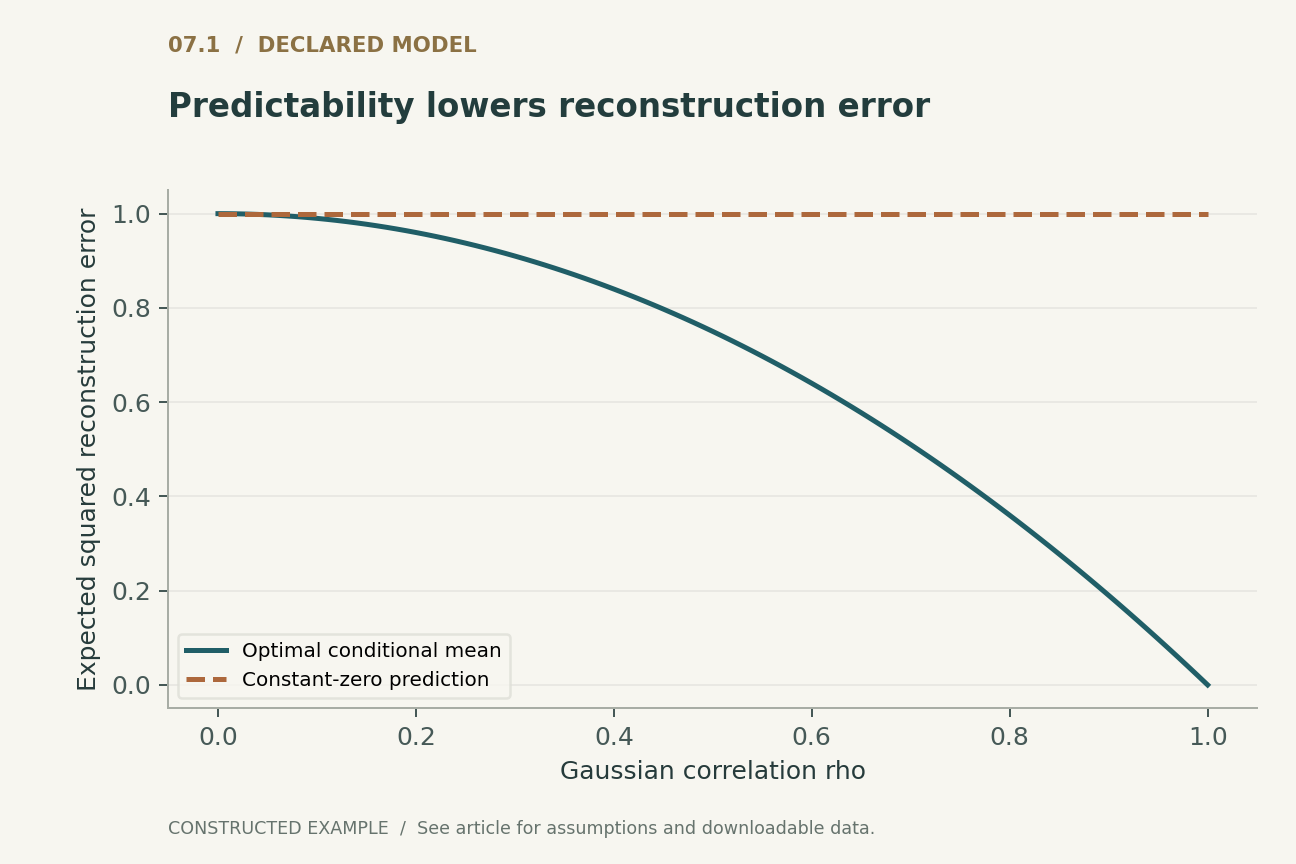
Let X and V be jointly Gaussian with zero mean, unit variance and correlation rho. Conditional prediction of X from V is rho times V, with mean squared error one minus rho squared. Panel 1 plots this irreducible error and compares it with a constant predictor whose error remains one. As correlation approaches one, the reconstruction problem becomes easy.
Now append an independent fair semantic bit Y to the unobserved state, while ensuring that neither X nor V depends on Y. Perfect prediction of X supplies no information about Y. This is an intentionally strict counterexample, not a model of all visual semantics: it disproves the universal implication from reconstruction quality to task information. To claim semantic transfer, one must show an actual dependency between the training signal and the target or measure the downstream decision directly. Replacing an independent bit with a weakly correlated one makes the conclusion quantitative rather than eliminating the distinction.
7. Masking can erase the only useful evidence
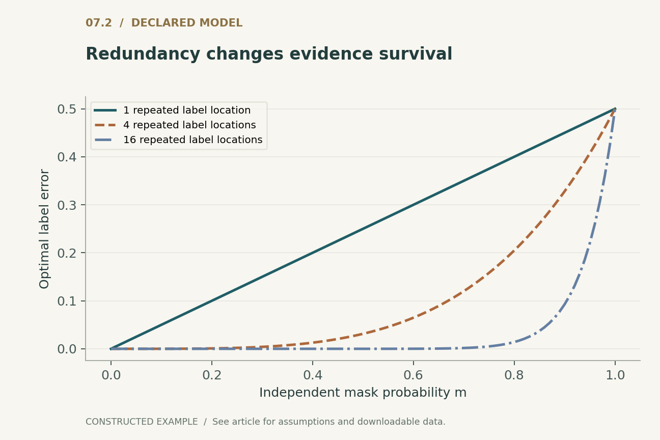
Consider a separate construction in which a fair label bit is copied into r distinct observable locations. Each location is independently masked with probability m. If at least one copy remains visible, the label can be decoded perfectly. If all copies disappear, the visible observation contains no label information and optimal classification must guess. Averaging these cases yields Bayes error equal to half of m raised to r.
Panel 2 compares one, four and sixteen copies. These curves quantify redundancy under independent masking, not the behavior of any trained vision model. At a masking probability of one half, four copies reduce the unavoidable error to one thirty-second. With one copy, it is one quarter. The same global masking fraction can therefore induce radically different supervision depending on how task information is distributed. Masking ratios should be discussed alongside semantic redundancy and spatial organization, not treated as portable constants that guarantee a suitably difficult learning task.
8. Correlated masks change the calculation
The repeated-bit formula depends on independent masking. If all copies lie inside one region removed by a block mask, their losses can be perfectly correlated: the probability of losing every copy can equal the region-removal probability rather than its rth power. A large numerical advantage from redundancy disappears when the mask couples the redundant locations.
This observation suggests a controlled comparison between independent patch masks and spatially contiguous masks at matched expected visible area. Matching only the mean count is insufficient; the joint distribution of visibility changes which relations are observable. The same issue occurs when important evidence sits near a crop boundary or within a repeated visual motif. A useful evaluation records the distribution of visible task evidence, ideally using a synthetic diagnostic with known causal factors before interpreting a real dataset. The proposed comparison does not assume one mask family will win; it identifies the mechanism that must be measured to explain a result.
9. Compute savings require a declared denominator
If an encoder processes N tokens and retains a deterministic fraction one minus m, the number of pairwise attention scores scales from N squared to N squared times one minus m squared. This is an operation-count comparison for that term, assuming divisibility and otherwise identical attention. It is not a wall-clock speed prediction.
Projection layers, feed-forward blocks, the decoder, data movement, optimizer work and padding can have different scaling. If masks are sampled independently and the visible count is random, its squared expectation also includes a variance term. A computation claim must state whether it uses a fixed visible count, an expected count approximation, or an actual execution trace. In this article the attention expression is deliberately limited to a fixed-count thought experiment, while the repeated-bit information calculation uses independent Bernoulli masking. These are separate models. Keeping their assumptions explicit prevents a convenient algebraic expression from becoming a misleading systems claim.
10. Decoder strength can move the burden
A powerful decoder may exploit spatial regularity or a learned prior even when the encoder exposes only coarse information. A weak decoder may force the encoder to make useful distinctions accessible, but it can also limit reconstruction without improving transfer. Neither direction is guaranteed by architecture size alone.
A diagnostic should vary decoder capacity while holding the encoder, visible information and training budget fixed. It should then measure downstream tasks using an explicitly specified readout. If reconstruction improves while transfer stagnates, the improvement may belong to the decoder or target modeling rather than a broadly better representation. If transfer improves while pixel error worsens, the target metric may emphasize details outside the downstream objective. These outcomes are not contradictions. They reveal that the two measurements refer to different computations. An experiment that discards the decoder after pretraining should evaluate the retained encoder directly rather than describing the quality of the discarded joint system as its final result.
11. A controlled semantics audit
A proposed audit should introduce independent controls for local texture predictability and task-relevant global structure. The Gaussian construction checks the first principle exactly; the repeated-bit construction checks evidence loss exactly. A larger synthetic dataset could combine textured backgrounds with objects whose labels depend on relations among separated parts, allowing mask geometry and target loss to be manipulated independently.
Real-image evaluation should then test tasks chosen before inspecting model outcomes. Reconstruction error, calibration of missing-content predictions, and downstream risk should be reported separately. A probe must declare its training data and capacity; full fine-tuning is a different intervention from a frozen representation. Repeated training runs should be the unit for optimization uncertainty. The supplied executable examples perform no neural training and cannot establish how often a particular shortcut appears in practice. Their purpose is to make proposed mechanisms falsifiable and expose which additional measurements would be required.
12. A defensible reconstruction claim
Reconstruction becomes scientifically informative when the target, visibility process, decoder access and loss are specified together. The resulting statement can be strong: the system accurately predicts a defined conditional target, or learns a representation that transfers to declared decisions under a stated protocol. The statement becomes weak when a proxy objective is silently renamed understanding.
The worked examples show two boundaries. Easy conditional prediction can coexist with complete absence of a semantic variable, and aggressive masking can remove all evidence required for a decision. Neither boundary invalidates masked pretraining. They explain why its empirical success requires careful interpretation and why transfer evaluation remains necessary. A productive next step is to report information-preservation audits alongside reconstruction curves, particularly for tasks whose decisive features occupy small or unusual regions. This would turn mask selection from an inherited recipe into a measurable assumption about what the representation should retain.
Executed locally · Bounded scope
Gaussian conditional risk and exhaustive label-mask enumeration
Second-moment algebra and exhaustive masks for up to eight repeated bits; no image reconstruction model is trained.
1191 assertions passed. These checks validate the supplied example, not the cited systems.
Inspect the recorded witness
{
  "gaussian_rho": 0.6,
  "optimal_mse": 0.64,
  "copies": 4,
  "mask_probability": 0.5,
  "label_error": 0.03125,
  "enumerated_copy_counts": [
    1,
    2,
    3,
    4,
    5,
    6,
    7,
    8
  ]
}
Example runner · Model loader · Training models · Representation models · Generation models · Reliability modelsRead the complete check results
A declared analytical model
Four equations, explicit assumptions
(1) Risk decomposition for square-integrable scalar X and measurable predictor g with finite risk.
(2) Joint Gaussian example for |rho| <= 1; endpoints are understood as degenerate Gaussian limits.
(3) Fair label repeated in r visible locations, independently masked with probability m; no other label evidence.
(4) Fixed visible token count, not Bernoulli masking; compares only dense attention-score pair counts, excluding decoder and other work.
Constructed examples · Reproducible data
Inspect the quantitative argument
These curves are calculated from the declared models. They are not observations from the cited studies. Every figure includes its numeric data and vector version.


Which evidence answers which question?
| Choice | Changes directly | Required separate measurement |
|---|---|---|
| Pixel squared error | Conditional mean target | Semantic transfer and uncertainty |
| Discrete-token prediction | Tokenizer-defined distinctions | Target omissions and tokenizer provenance |
| Independent patch masks | Joint visibility distribution | Evidence survival and mask correlations |
| Encoder-only visible tokens | Encoder operation count | End-to-end latency and retained representation quality |
A proposed validation protocol
This is a proposed evaluation design. No production-system or hardware benchmark was performed. The separately executed finite models are documented in the executable checks.
- Specify missing targets, decoder inputs, mask distribution and downstream labels.
- Verify Gaussian conditional-risk identities and repeated-bit Bayes errors independently.
- Match expected visible area while varying independent and contiguous masking.
- Manipulate nuisance predictability separately from semantic redundancy.
- Vary decoder capacity and evaluate the frozen encoder with prespecified probes.
- Report reconstruction, transfer, compute accounting and uncertainty as distinct outcomes.
What the primary sources establish
Pascal Vincent, Hugo Larochelle, Yoshua Bengio et al. · 2008 [1]
Contribution. Corrupted-input reconstruction is used to learn representations and initialize deep architectures.
Boundary. Its experiments do not establish universal usefulness of arbitrary corruptions.
Source locator. Training principle and experimental sections.
Kaiming He, Xinlei Chen, Saining Xie et al. · 2022 [2]
Contribution. MAE separates a visible-patch encoder from a reconstruction decoder.
Boundary. Mask ratios and measured efficiency are specific to the evaluated setup.
Source locator. Abstract and architecture description.
Hangbo Bao, Li Dong, Songhao Piao et al. · 2021 [3]
Contribution. BEiT predicts discrete visual targets from corrupted image patches.
Boundary. The target tokenizer is part of the method; this review inspects the revised preprint.
Source locator. Abstract and masked image modeling description.
Limits of this analysis
- The exact models isolate logical boundaries rather than realistic image statistics.
- Squared error is only one reconstruction objective; perceptual and likelihood losses require separate analysis.
- No MAE, BEiT or denoising-autoencoder benchmark was reproduced.
- Semantic labels and their relevance remain task definitions, not quantities identified by an unlabeled reconstruction loss.
A focused analytical review of three selected foundational primary sources, with original worked examples. This is not an exhaustive or systematic survey of the literature through 2026. Source access and version notes are recorded with the bibliography.
Questions that would change the conclusion
- Can masking policies be selected from a measurable evidence-survival criterion for several downstream tasks?
- How much useful transfer comes from the encoder versus structure supplied by the reconstruction target?
- Which evaluations distinguish calibrated uncertainty about missing content from merely plausible completions?
References
- Pascal Vincent, Hugo Larochelle, Yoshua Bengio et al.. Extracting and Composing Robust Features with Denoising Autoencoders. Proceedings of the 25th International Conference on Machine Learning (2008). 10.1145/1390156.1390294.
- Kaiming He, Xinlei Chen, Saining Xie et al.. Masked Autoencoders Are Scalable Vision Learners. Proceedings of the IEEE/CVF Conference on Computer Vision and Pattern Recognition (2022). Primary source.
- Hangbo Bao, Li Dong, Songhao Piao et al.. BEiT: BERT Pre-Training of Image Transformers. arXiv (2021). 10.48550/arXiv.2106.08254.
Source [1] access. Primary paper PDF text and primary bibliographic landing page inspected.
Version note. Author-hosted Toronto PDF inspected; Montreal mirror denied automated access.
Source [2] access. Primary paper PDF text and primary bibliographic landing page inspected.
Source [3] access. Primary paper PDF text and primary bibliographic landing page inspected.
Version note. This bibliography cites the 2021 preprint identifier. The inspected PDF/landing page is revision v2 dated 3 September 2022; no conference-version identity is assumed.
Bibliographic identities were checked against primary publisher and author records. Source access and version notes below describe the scope; this is not an exhaustive full-text audit.
Authorship and provenance
Written and technically self-reviewed by Codex (AI). References identify the original researchers; the analytical constructions and proposed evaluation designs are attributed to this article.
Covers are conceptual ImageGen illustrations. Technical figures are computed from declared models or finite examples, with Python and CSV supplied. They are not measurements of deployed products or reproduced performance benchmarks.
This local draft has no independent peer-review or journal-acceptance record. Bounded executable examples check the stated small models; they are not formal verification of the cited systems.