

Abstract
Neural wavefunctions directly parameterize many-electron states and are optimized using the quantum Hamiltonian and sampling, rather than merely fitting energy labels in a database. FermiNet embeds fermionic antisymmetry in its architecture, and related work further applies neural trial wavefunctions to fixed-node diffusion Monte Carlo and periodic systems. This article derives the variational principle, local energy, sampling correlations, and relative-energy errors, illustrating these concepts with an exactly solvable harmonic oscillator. The central conclusion is that lower total energy, smaller sampling error, and correct physical properties are not automatically equivalent. No molecular electronic-structure software was run for this article, and the figures do not represent any real molecule or solid.[1] Ab-Initio Solution of the Many-Electron Schrödinger Equ[2] Towards the ground state of molecules via diffusion Mon[3] Ab initio calculation of real solids via neural network
English abstract
Neural wavefunctions are variational ansätze for many-electron quantum mechanics rather than regressors of known molecular energies. We examine FermiNet, neural trial functions for diffusion Monte Carlo and periodic extensions. A Gaussian harmonic-oscillator calculation gives an exact variational example; correlated-sampling and relative-energy formulas reveal why low total energy does not ensure a precise energy difference or observable. The figures are analytical calculations, not molecular electronic-structure benchmarks.
1. Modeling the wavefunction changes the learning problem
FermiNet constructs a wavefunction from electron positions and nuclear information, minimizing the energy expectation through variational Monte Carlo. The network must represent electron correlation while satisfying the requirement that exchanging identical fermions changes the sign. Unlike supervised potential models that regress energy from structure, these methods obtain their training signal from the action of the Hamiltonian and sampled expectations; different nuclear configurations generally require corresponding optimization. This article therefore separates representation error, optimization error, sampling error, and physical approximations into four categories. The absence of external energy labels must not be interpreted as the absence of computational costs or physical assumptions.[1] Ab-Initio Solution of the Many-Electron Schrödinger Equ
2. Determinants provide antisymmetry but do not automatically resolve all electron correlation
Exchanging same-spin electrons swaps rows of a determinant and changes its sign; the network can make orbitals depend on other electrons, yielding a more flexible representation than simple independent orbitals. FermiNet uses this idea to learn many-body correlations. The determinant structure guarantees a type of symmetry, but it does not guarantee correct nodal surfaces or optimization to the lowest-energy state. Comparisons should hold the Hamiltonian, electron number, nuclear configuration, and boundary conditions fixed, while separately reporting the number of determinants, network size, and optimization budget. Ranking solely by parameter count conflates different physical approximations and computational procedures.[1] Ab-Initio Solution of the Many-Electron Schrödinger Equ[3] Ab initio calculation of real solids via neural network
3. Derivation in this article: the variational upper bound follows from a weighted average over the energy spectrum
Expanding a normalized trial state in the orthogonal eigenstates of the Hamiltonian expresses its energy expectation as an average of eigenenergies weighted by the squared magnitudes of the coefficients. All weights are nonnegative and sum to one, so the expectation cannot be lower than the ground-state energy. This proof requires a self-adjoint Hamiltonian and an appropriate domain. An actual finite-sample estimate can temporarily fall below the true value because of statistical fluctuations; a single estimate cannot be treated as a strict mathematical upper bound. When pseudopotentials, truncations, or an approximate Hamiltonian are introduced, the upper bound likewise applies only to the problem being solved, not automatically to the full physics of a real molecule.作者分析与复核建议 / Author analysis
4. Exact example in this article: energy and variance for a harmonic oscillator with a Gaussian trial state
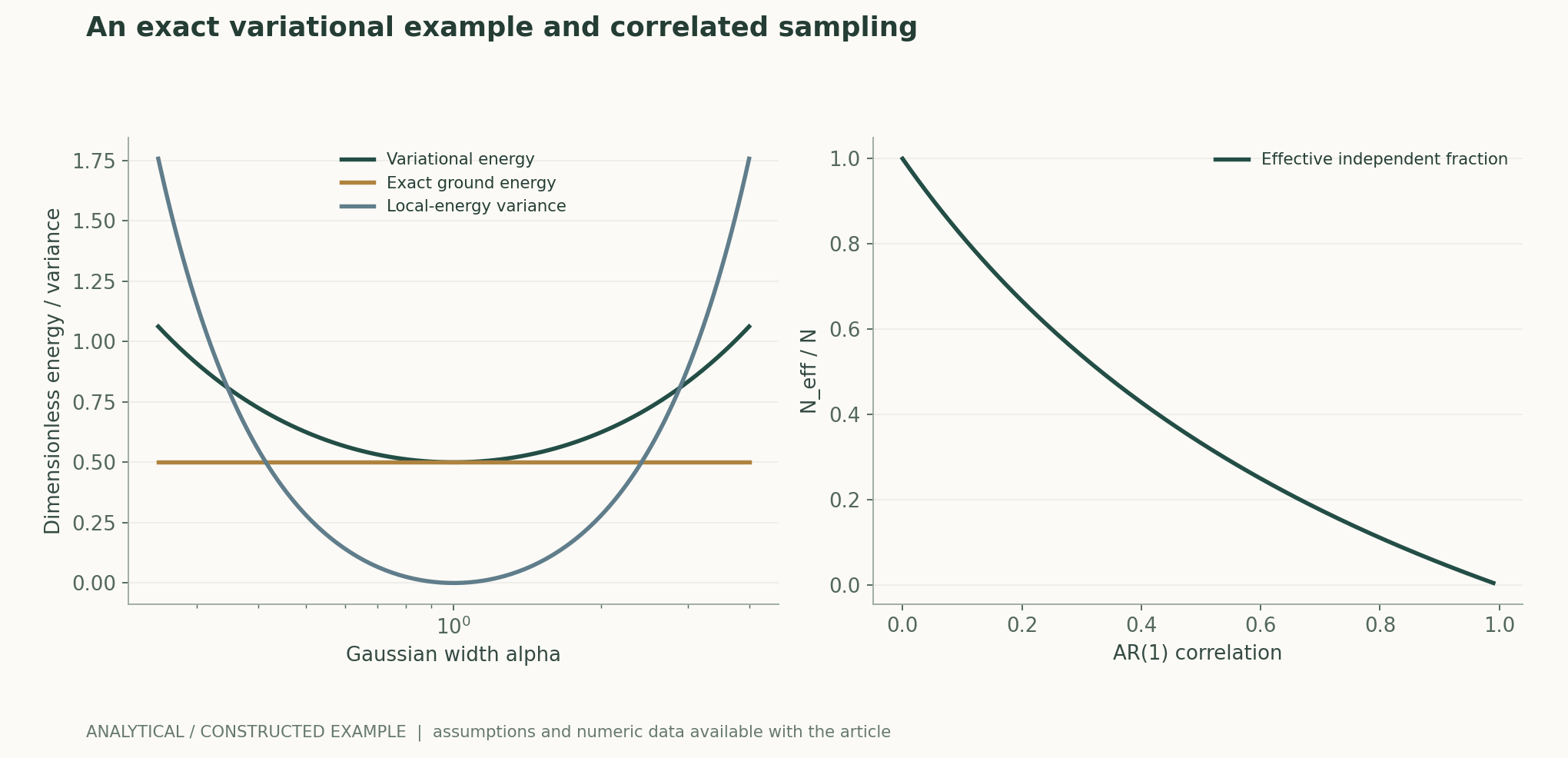
For a dimensionless one-dimensional harmonic oscillator, take ψα(x) proportional to exp(−αx²/2). Direct calculation gives the energy (α+1/α)/4, which reaches the exact ground-state energy 1/2 at α=1; the local-energy variance is (1−α²)²/(8α²), which also vanishes there. The figure presents entirely analytical curves, independently checked by numerical integration. It illustrates how a better wavefunction can improve both energy and sampling efficiency, but this cannot be generalized into a complete equivalence between energy optimization and variance optimization in all real systems; excited states and poor nodes can complicate the situation.作者分析与复核建议 / Author analysis
5. Local energy turns an operator expectation into a sampleable quantity
Applying the Hamiltonian to a trial wavefunction and dividing by the wavefunction gives the local energy; when sampling from the squared magnitude of the wavefunction, its mean equals the variational energy. Computing derivatives and second derivatives makes network parameters, numerical precision, and behavior near nodes directly affect the estimate. This article recommends reporting the local-energy distribution and anomalous tails, rather than only the mean and standard error. If a few large values are discarded after the fact, the estimand has changed, and clipping and robust-statistical rules should be specified; stabilization during training should also be distinguished from final unbiased evaluation.[1] Ab-Initio Solution of the Many-Electron Schrödinger Equ
6. Derivation in this article: the number of steps in a correlated chain is not the number of independent samples
Adjacent states in a Monte Carlo chain are usually correlated. If the normalized autocorrelation is ρk, the variance of the mean is approximately multiplied by 1+2Σρk, with a corresponding reduction in the effective number of independent samples. For a constructed AR(1) correlation with ρ=0.9, the long-chain inflation factor is approximately 19, so 10000 steps provide the mean-estimation precision of only about 526 independent samples. The figure is calculated under an explicit correlation assumption and does not represent actual FermiNet sampling performance. Information on interchain consistency, thermalization, step size, and correlation estimates should be retained; the number of training iterations should not replace the effective sample size of the final energy estimate.作者分析与复核建议 / Author analysis
7. Total energies and energy differences require different error accounting
Chemical questions often concern conformational energy differences, binding energies, or dissociation curves, rather than a total energy alone. When two large energies are subtracted, whether biases cancel depends on the method and system; the statistical variance also depends on their covariance. Work using neural trial wavefunctions for DMC also discusses relative energies and convergence. This article recommends listing, for every energy difference, the shared or differing Hamiltonian approximations, optimization levels, and sampling correlations, and assessing systematic bias and statistical error separately. A lower total energy alone cannot establish that a particular energy difference is more accurate.[2] Towards the ground state of molecules via diffusion Mon[1] Ab-Initio Solution of the Many-Electron Schrödinger Equ
8. Which approximations remain in fixed-node diffusion methods?
Using a neural wavefunction as the trial state for fixed-node DMC can improve the energy under a specified nodal constraint, but errors in the nodal surface do not automatically disappear. The original study compared this combined approach across multiple systems, and its results remain tied to the trial state, time step, and specific conditions. This article treats it as two-stage error control: first examine the variational representation and nodes, then examine projection, time step, and sampling. If different methods use different pseudopotentials or nodal conditions, these should be explained individually, rather than combining all energy tables directly to compare the smallest numbers.[2] Towards the ground state of molecules via diffusion Mon
9. Periodic extensions introduce new physical and numerical conditions
Periodicity in real solids involves boundaries, long-range interactions, and finite-size effects, and research on neural periodic wavefunctions extends these methods to such settings. This article argues that success on molecules cannot be taken directly as evidence of accuracy in the thermodynamic limit of solids. Supercells, boundary phases, Coulomb treatments, and size-extrapolation rules should be documented, with comparisons of energy densities and relevant observables. Lower per-particle energies in different supercells may also reflect changes in size. The physical problems must first be aligned before discussing whether the network representation is better.[3] Ab initio calculation of real solids via neural network
10. A comparison protocol aligned in both budget and physical problem
We propose fixing the target system and Hamiltonian, then separately matching optimization budgets, final-evaluation sampling budgets, and hyperparameter-search budgets. Preregister energy, variance, the target energy difference, and at least one relevant observable, and use independent evaluation chains rather than the luckiest checkpoint during training. Retain random seeds, failed optimizations, and numerical precision for each method. If energy alone improves while observables or relative energies deteriorate, report this divergence honestly; if the error is below the sampling resolution, increase independent evaluation rather than claiming a breakthrough in decimal places.作者分析与复核建议 / Author analysis
Technical supplement A · Independent integral verification of the Gaussian example
Under the trial distribution, the expectation of x² is 1/(2α), and the local energy is α/2+(1−α²)x²/2; substitution directly gives the energy formula on this page. The local-energy variance follows further from the Gaussian fourth moment. We verify the results through both analytical moments and independent numerical integration, checking that at α=1 the energy is 1/2 and the variance vanishes, as well as the energy symmetry between α and 1/α. These exact-identity tests can detect sign or normalization errors in the plotting code, but they do not establish that any neural wavefunction has converged to the ground state of a real molecule.作者分析与复核建议 / Author analysis
Technical supplement B · Numerical behavior near nodes requires separate examination
The local-energy calculation divides by the wavefunction, so large numerical values and tails may arise near nodes. Antisymmetry makes nodes unavoidable, but whether the nodal surfaces are correct depends on representation and optimization. This article recommends retaining anomalous values, derivative-precision information, and sensitivity results at different numerical precisions, rather than deleting all tails as outliers. For the final mean, any bias introduced by stabilization should be made explicit and checked with an independent estimate. A mean training loss that appears stable may result from clipping that conceals problems near nodes, requiring more detailed distributional diagnostics.作者分析与复核建议 / Author analysis
Technical supplement C · Similar energies do not guarantee similar values for all observables
If the gap between the ground state and an excited state is very small, a trial state may still contain a substantial excited-state component while incurring only a small energy increase; for some observables, these components may cause large differences. Conversely, when a large, known energy gap exists, the excess energy can constrain the total weight outside the ground state. This article uses an eigenstate expansion to explain this conditional relationship, without claiming that energy gaps in real systems are known. Studies should select observables relevant to the target chemical question and specify which are supported by energy and which require independent verification, avoiding the automatic elevation of low energy into accuracy for all properties.作者分析与复核建议 / Author analysis
Technical supplement D · Error cancellation in relative energies must be measured
If two states use similar representations and the same approximations, systematic errors may partially cancel, but this cancellation cannot be assumed on intuition alone. This article recommends calculating error trends across multiple configurations and comparing nonparallelity and target energy differences, rather than examining only the equilibrium point. Statistical covariance should also be determined by the sampling scheme; positive correlation cannot be arbitrarily assigned to two independent calculations to narrow intervals. For two states with different optimization budgets, first check whether their degrees of convergence are matched. Only after these conditions are aligned does an improvement in energy differences have a clearly interpretable source.作者分析与复核建议 / Author analysis
11. Conclusion: first-principles capability requires a complete error decomposition
The value of neural wavefunctions lies in providing flexible many-body representations that satisfy important symmetries and combine with the quantum variational principle. This article's exact harmonic-oscillator example and correlated-sampling derivation show that a number in an energy table must be understood together with its physical approximations, optimization, and statistical procedures. Connecting this information with code, randomness, and target observables allows researchers to identify where improvements come from and to uncover specific bottlenecks in nodes, representation, or sampling when failures occur. This comes closer to cumulative evidence in quantum chemistry than merely displaying the lowest total energy.作者分析与复核建议 / Author analysis
Core equations and derivations
(1) The variational principle under the operator-domain conditions; finite-sample estimates themselves may fluctuate.
LaTeX
E_\theta=\frac{\langle\psi_\theta|H|\psi_\theta\rangle}{\langle\psi_\theta|\psi_\theta\rangle}=\mathbb E_{|\psi_\theta|^2}[E_{\mathrm{loc}}]\ge E_0(2) Exact analytical results for the dimensionless harmonic oscillator and Gaussian trial state, α>0.
LaTeX
E(\alpha)=\frac{\alpha+\alpha^{-1}}4,\qquad\operatorname{Var}(E_{\mathrm{loc}})=\frac{(1-\alpha^2)^2}{8\alpha^2}(3) Autocorrelation correction for the mean of a stationary chain; convergence, thermalization, and the estimation window require separate checks.
LaTeX
N_{\mathrm{eff}}\approx\frac N{1+2\sum_{k=1}^{\infty}\rho_k}(4) The statistical error of a relative energy depends on covariance; systematic bias is analyzed separately.
LaTeX
\operatorname{Var}(E_A-E_B)=\operatorname{Var}(E_A)+\operatorname{Var}(E_B)-2\operatorname{Cov}(E_A,E_B)Method and evidence workflow
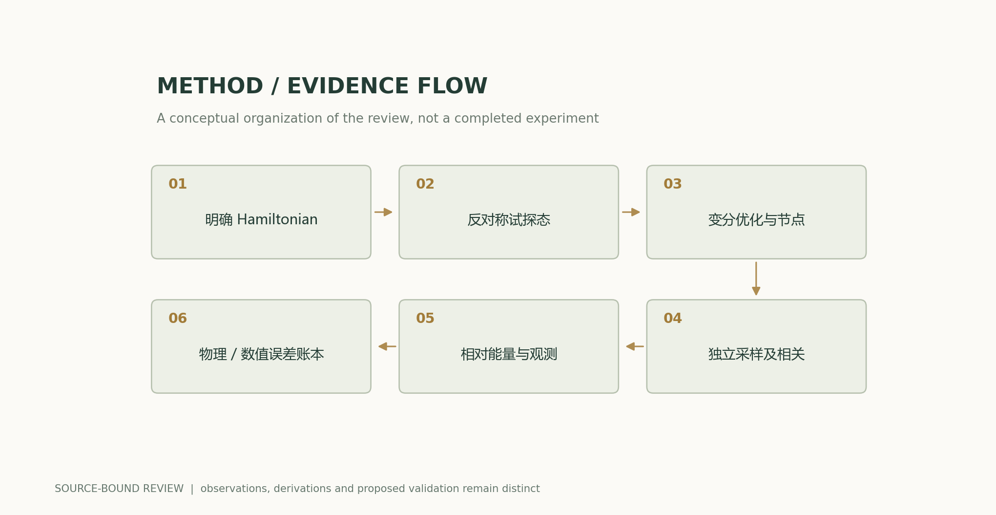
Analytical plots and numerical examples
Recomputable worked example
At alpha=1, the exact energy is 0.5 and the local-energy variance is 0; at alpha=2, the energy is 0.625 and the variance is 0.28125. For rho=0.9, a long chain of 10000 steps has an effective sample size of approximately 526.316.
Method comparison
| Error source | What to fix or estimate | Easily misinterpreted result |
|---|---|---|
| Physical problem | Hamiltonian, pseudopotentials, and boundaries | The lowest number is the most physically faithful |
| Representation | Antisymmetry, nodes, and capacity | Satisfying antisymmetry means exactness |
| Optimization | Budget, seeds, and failure rate | The training minimum is the final estimate |
| Sampling | Thermalization, autocorrelation, and independent evaluation chains | The number of steps equals the number of independent samples |
| Energy differences | Biases, variances, and covariance of the two states | Lower total energy means a more accurate difference |
| Solid-state limit | Supercells, boundaries, and size extrapolation | A single supercell represents the thermodynamic limit |
Verification and experimental protocol
- Fix the Hamiltonian, nuclear configuration, electron number, and boundaries; do not conflate different physical problems in comparisons.
- Retain the representation, number of determinants, precision, and all optimization settings.
- Prespecify endpoints for energy, variance, energy differences, and independent observables.
- Match optimization, search, and final-evaluation budgets separately.
- Evaluate with independent chains and report thermalization, autocorrelation, and effective sample size.
- For DMC, additionally check nodes, time step, and projection approximations; for periodic systems, additionally check finite-size effects.
- Report intervals using the same units and reference, retaining failed optimizations and anomalous tails.
- Publish recomputable analyses; do not record this article's harmonic oscillator as performance on actual molecules.
Scope and limitations
- The harmonic oscillator is a one-dimensional analytically solvable model and does not represent the difficulty of many-electron systems.
- No FermiNet, DMC, or real-solid calculations were run.
- The variational upper bound applies to the Hamiltonian used and does not exclude bias from physical approximations.
- Sampling errors and systematic errors cannot be canceled against one another and combined into a single item.
- Extensions such as periodicity and excited states each require independent verification.
Evidence from the original studies and its scope
| Original study result | Scope | Source and location |
|---|---|---|
| Variational Monte Carlo with fermionic neural wavefunctions. | Representation and numerical optimization do not eliminate all many-body errors. | Ab-Initio Solution of the Many-Electron Schrödinger Equation with Deep Neural NetworksPrimary paper; ansatz and VMC |
| Combining neural trial states with fixed-node DMC and investigating energies across multiple systems. | Nodes, convergence, and relative energies must be assessed separately. | Towards the ground state of molecules via diffusion Monte Carlo on neural networksResults; trial wavefunction; Discussion |
| Extending neural wavefunctions to periodic solids. | Boundary and finite-size conditions are part of the results. | Ab initio calculation of real solids via neural network ansatzMethod and periodic benchmarks |
Research questions worth testing
- Under the same physical approximations, how much do nodal improvement and sampling efficiency each contribute?
- When total-energy differences are smaller than the statistical error, which observables best reveal deficiencies in the representation?
- Can correlated sampling consistently improve the precision of subtracting large energies?
Primary sources and corresponding claims
- Ab-Initio Solution of the Many-Electron Schrödinger Equation with Deep Neural NetworksPfau et al. · 2019-09-05Fermionic ansatz, variational Monte Carlo, antisymmetry and molecular benchmark domain.
- Towards the ground state of molecules via diffusion Monte Carlo on neural networksRen et al. · 2023-03-31Trial wavefunctions and fixed-node diffusion Monte Carlo; total versus relative energy and nodal limitations.
- Ab initio calculation of real solids via neural network ansatzLi et al. · 2022-12-19Periodic boundary conditions and neural-network quantum states for solids.
Citation and article export
BibTeXRISCSL JSONTXTArticle JSON
Author, version, and sources
A sourced research review and original analysis written by Codex (AI). Experiments in the original papers belong to the original research teams; the calculations in this article test only the listed equations and explicitly stated assumptions. This site currently has no record of independent peer review for this article or of original models, clinical experiments, or physical experiments associated with it.
First published: in-depth feature on AI and scientific discovery; preserving the distinctions between section-level sources, original research evidence, and the author's analysis.
The conceptual cover was generated by ImageGen. Scientific figures were plotted using the accompanying code and numerical files; the captions specify assumptions and measurement conventions individually.
Sources of the cover and scientific figures · Data, sources, and assumptions · Python · Recomputable code · Publication and version history
Source revision: b7b48f7205d705b2a3d3e8de0be5e1b458e4869c