
Abstract
Spatial omics connects cellular states with tissue structure, but different methods produce different outputs: some align cells with spatial locations, some estimate local cell composition, and others learn representations that can predict neighborhoods. This article compares Tangram, CytoSPACE, and Nicheformer using mixture-signal identifiability and neighborhood scale as a common framework. We derive the error amplification caused by nearly collinear markers and use a constructed tissue to show how changing the radius alters neighborhood composition. The central assessment is that low expression reconstruction error does not guarantee a unique cell mapping, and proximity alone cannot establish cell communication. No real tissues or patient samples were used in the figures and tables.[1] Deep learning and alignment of spatially resolved singl[2] High-resolution alignment of single-cell and spatial tr[3] Nicheformer: a foundation model for single-cell and spa
English abstract
Spatial models connect cellular expression to tissue organization, but cell placement, local composition and communication are distinct inference problems. We compare Tangram, CytoSPACE and Nicheformer through an identifiability lens. A two-signature mixture and a radius-dependent neighborhood example expose ambiguity that can persist despite low reconstruction error. We propose blocked spatial validation, held-out genes and specimen-level replication to distinguish useful interpolation from transferable tissue biology.
1. Three different problems may underlie the same tissue map
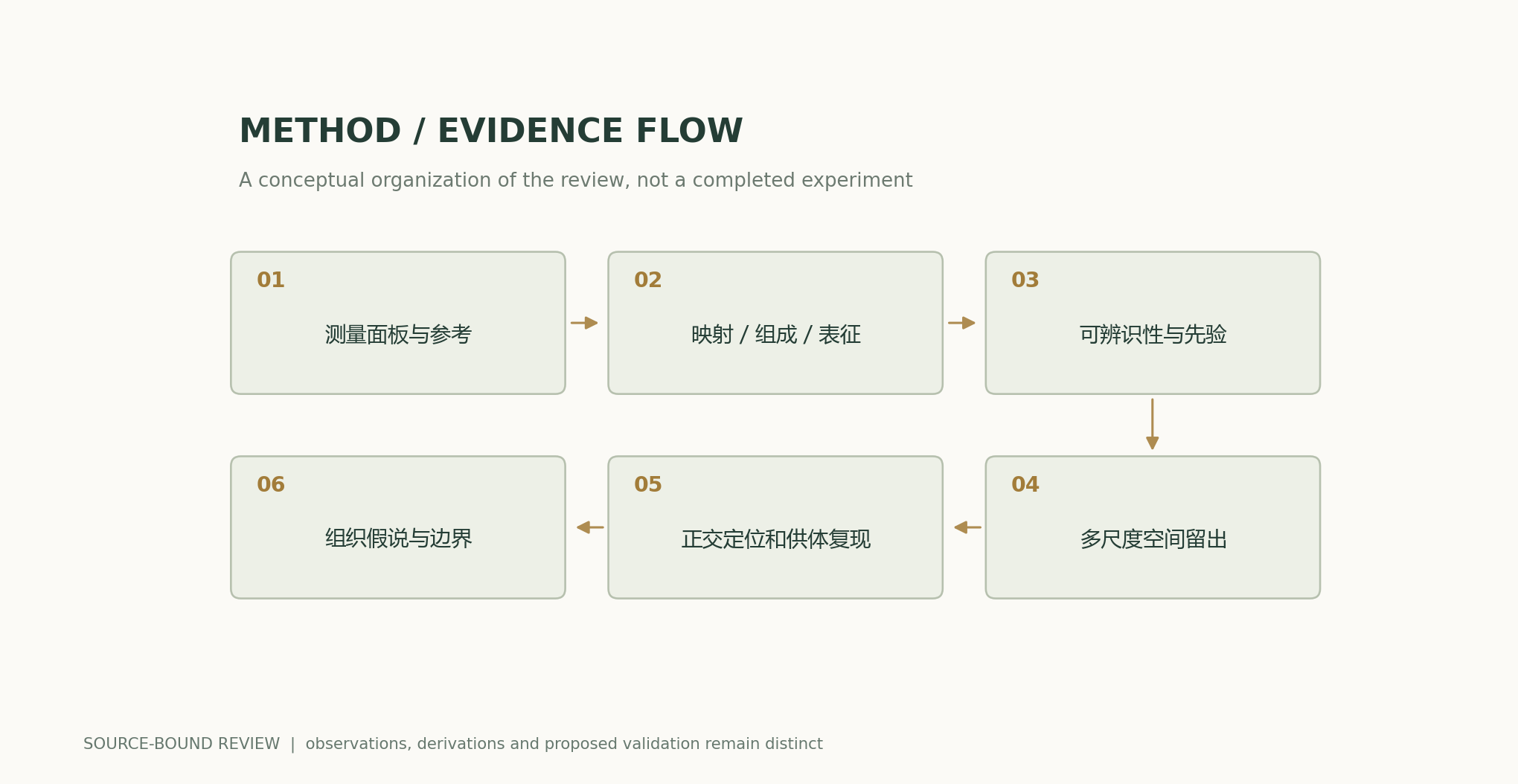
Tangram aligns single-cell expression with spatial observations, CytoSPACE investigates high-resolution assignment of cells to spatial locations, and Nicheformer learns transferable representations from single-cell and spatial data. These methods should not be ranked solely by a spatial heatmap that looks clear. Mapping concerns location and assignment, composition concerns the proportions of cell types within a region, and representation concerns which downstream tasks an embedding can support. This article recommends first establishing a dictionary of output units—single cells, measurement spots, neighborhoods, or tissue regions—and then specifying which variables are actually observed and which are completed by priors or models.[1] Deep learning and alignment of spatially resolved singl[2] High-resolution alignment of single-cell and spatial tr[3] Nicheformer: a foundation model for single-cell and spa
2. Expression alignment can exploit shared genes but is also constrained by measurement coverage
Tangram's method description emphasizes shared genes and compatible tissue sources; mapping optimization makes reconstructed expression agree with spatial observations. If the measurement panel lacks markers that distinguish similar cell states, different assignments may produce nearly identical expression. This article treats this as an identifiability problem rather than simply attributing it to insufficient network capacity. The gene panel, capture differences, and reference cell composition must be retained; when a cell type is absent from the reference, the model may explain it using the closest known type. Validation should include markers not used for fitting and external morphological or localization evidence, rather than merely reevaluating training genes.[1] Deep learning and alignment of spatially resolved singl[2] High-resolution alignment of single-cell and spatial tr
3. Derivation in this article: how similar cell signatures amplify composition errors
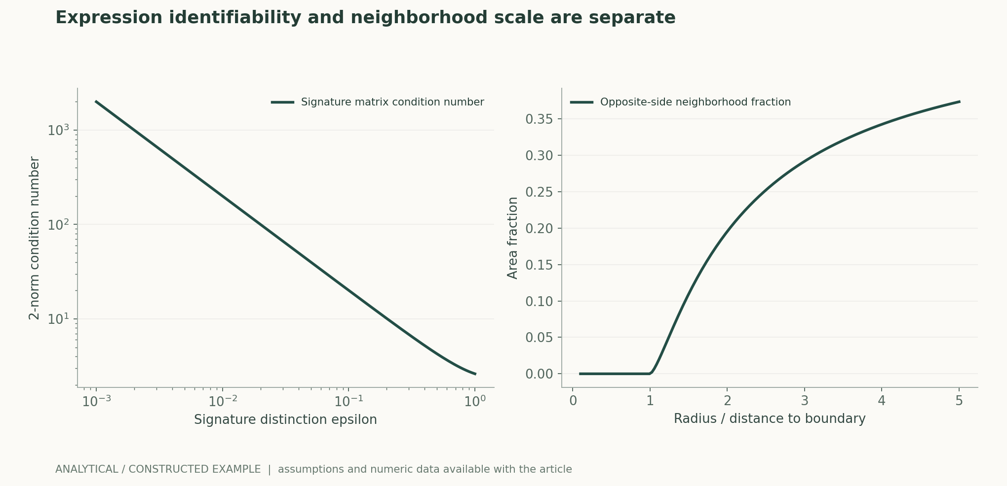
Let the two normalized cell signatures be a first =(1,0) and a second =(1,ε), with measurements formed by mixing them in proportions. The second component provides only ε times the discriminating signal, so the same observational perturbation δ corresponds to a composition change of approximately δ/ε. When ε decreases from 1 to 0.01, the measurement precision required to distinguish the same difference in proportions increases one hundredfold. If ε=0, the two signatures are identical, and composition is no longer unique. The figure shows how the matrix condition number and recovery error vary with ε; all units and errors are constructed values. It explains why a larger model cannot recover a unique answer from information that does not exist.作者分析与复核建议 / Author analysis
4. Composition constraints can narrow the feasible set but may also introduce bias
CytoSPACE formulates cell mapping as an optimization problem with constraints on composition and other quantities, demonstrating that the task can use information beyond expression. This article analyzes the general implication: known cell counts or proportions can exclude many implausible assignments, but the constraints themselves may be wrong if the priors come from a different section, donor, or technology. Unconstrained fitting error, constraint deviation, and external localization accuracy should be reported separately, with sensitivity analyses for perturbations to the priors. If a model works only when exact ground-truth proportions are known, its capability should be described as conditional mapping, not as independently discovering the entire cell composition from raw spatial signals.[2] High-resolution alignment of single-cell and spatial tr
5. Neighborhood representations turn a spatial problem into a scale problem
Nicheformer uses local neighborhood composition as one of its interpretable tasks and evaluates it across multiple neighborhood scales and tissue datasets. A fixed radius defines an explicit target, but a small radius emphasizes immediate proximity, whereas a large radius more closely reflects the regional environment; the two may address different biological questions. This article recommends treating radius, boundary handling, cell density, and cell-type granularity as part of the results. In tissues of different densities, the same radius contains different numbers of cells; defining neighborhoods by a fixed number of nearest neighbors instead changes the physical distance. The most favorable scale must not be selected only after a significant result has been found.[3] Nicheformer: a foundation model for single-cell and spa
6. Analysis in this article: neighborhood composition changes with boundaries and radius
Construct a planar tissue with uniform cell density, with type A and type B cells on opposite sides of a straight boundary and a center located a distance d to the right of the boundary. When the radius satisfies r≤d, the neighborhood consists entirely of the right-hand type; when r>d, the proportion on the other side is determined by the area of a circular segment. Even if the central cell's expression remains completely unchanged, the neighborhood label changes continuously as the radius increases beyond d. This shows that some so-called “prediction errors” may arise from a mismatch in label scale. The figure gives exact circular-area proportions, not randomly placed cells or inference from real tissue; at the boundary, the limiting proportions are half on each side, while far from the boundary the proportion on the other side is zero.作者分析与复核建议 / Author analysis
7. Spatial correlation can make random splits overly optimistic
Adjacent locations within the same tissue section share microenvironments, batches, and measurement artifacts. If training and test spots are randomly split in an interleaved pattern, the model can exploit nearby similar patterns without necessarily learning rules that transfer across regions. This article proposes holding out contiguous spatial blocks, followed by stronger holdouts by section and donor, while retaining performance curves against distance from the training region during evaluation. Confidence intervals require resampling at least at the section or donor level, rather than treating every adjacent cell as an independent replicate. Random splits can still estimate local interpolation, but they must be reported under that name and cannot represent generalization to new tissues.作者分析与复核建议 / Author analysis
8. Colocalization and communication require different evidence
Spatial proximity between two cell types can support their presence in similar environments, but it cannot independently establish that a particular ligand–receptor axis is transmitting signals. Expression, protein, contact, and functional changes represent different observational levels. This article advocates storing colocalization statistics separately from mechanistic hypotheses: the former require control for cell abundance and tissue structure, while the latter must be able to exclude explanations involving a shared environment or a third cell type. If map changes primarily arise from changes in cell segmentation or type labels, the measurement pipeline should be corrected first, rather than attributing all changes to biological communication.作者分析与复核建议 / Author analysis
9. Establishing testable comparisons across technologies
A rigorous comparison should hold the tissue region, shared gene set, and reference conditions constant and test mapping, composition, and neighborhood tasks separately. Fitting genes and validation genes must be separated, and the priors that models are allowed to use should also be specified in the protocol. Primary endpoints could be localization or composition errors validated by independent markers, with regional transfer and rare-type performance as secondary endpoints. If a method excels on broad cell classes but assigns rare states to nearby major classes, this should be reported at the type level rather than concealed by an average weighted by overall cell counts.作者分析与复核建议 / Author analysis
Technical supplement A · From probabilistic mapping to single-cell assignment
A soft mapping matrix allows a cell to have weights at multiple locations; satisfying expression reconstruction does not mean that every cell already has a unique destination. Subsequently converting to hard assignments by taking the largest weight discards uncertainty and may change regional counts. This article recommends publishing summaries of soft weights, final assignments, and the differences between them together, and checking whether low-confidence objects cluster at boundaries or among similar types. If repeated optimizations yield different cell locations but the same regional composition, stable conclusions should be restricted to the composition level rather than forcibly treating every location as a confirmed single-cell fact.[1] Deep learning and alignment of spatially resolved singl[2] High-resolution alignment of single-cell and spatial tr
Technical supplement B · Distinguishing condition numbers from model misspecification
The linear perturbation bound assumes that the signature matrix A is known; if the actual reference comes from another technology or lacks states, the matrix itself also contains error. Observational and reference errors can then jointly alter composition, and reducing measurement noise alone may not resolve the problem. This article recommends varying reference cells, the gene panel, and count depth separately to examine output stability. If error primarily arises from missing reference states, increasing the number of samples from the same reference may merely make the wrong answer more confident. What is needed is additional discriminating information or allowance for an unknown class, rather than simply greater network capacity.作者分析与复核建议 / Author analysis
Technical supplement C · Neighborhood composition labels are subject to compositional constraints
The proportions of all types within a neighborhood sum to one, so an increase in one type forces other proportions down even if their absolute counts remain unchanged. Correlations between proportions therefore do not imply mutual exclusion between cells. This article recommends retaining both the total neighborhood cell count and type proportions, and distinguishing density from composition in the analysis. For zero proportions, it is also necessary to state whether they reflect genuine non-detection, an inability of the panel to distinguish the type, or the absence of neighborhood cells. Adding a pseudocount to every zero before computing correlations may change conclusions about rare types; pseudocounts and transformations should be included in an auditable configuration.作者分析与复核建议 / Author analysis
Technical supplement D · Registration across sections is not repeated measurement of the same cells
Adjacent sections can provide similar tissue contexts, but they do not always permit one-to-one correspondence for every cell. This article recommends dividing cross-section validation into regional, type, and cell granularities and retaining errors for each kind of correspondence. If only regional matching is available, model improvements should be reported using regional endpoints. Mixing precise cell-level coordinates with regional labels creates spurious high-resolution confirmation. For conclusions that depend on boundaries, registration can be deliberately shifted or perturbed to test whether they persist within an explicit range, rather than using only a single most favorable registration.作者分析与复核建议 / Author analysis
10. Conclusion: tissue ecology requires predictions with explicit scales
An important potential of spatial foundation models is to place cellular states back into their tissue environments, but credibility depends on explicitly defining the output target, available information, and scale. The two counterexamples in this article show, respectively, that expression identifiability and neighborhood definitions can both limit the uniqueness of an answer. Scientific deliverables should include the gene panel, reference, priors, spatial splits, and failure regions, so that subsequent reproduction can determine whether differences arise from technology, conditions, or biology. Binding these conditions to exact versions contributes more to accumulating transferable tissue knowledge than continually adding attractive heatmaps.作者分析与复核建议 / Author analysis
Core equations and derivations
(1) A general linear mixing example; actual capture, count, and expression models may be more complex.
LaTeX
y=A\pi+\eta,\qquad \pi_k\ge0,\quad\sum_k\pi_k=1(2) An unconstrained least-squares perturbation bound for fixed A with full column rank; constrained and misspecified cases require separate analysis.
LaTeX
\|\delta\pi\|\le\|A^+\|\,\|\delta y\|(3) The area proportion on the other side when a circular neighborhood crosses a straight boundary in a uniform plane; it is 0 when r≤d.
LaTeX
q(r,d)=\frac{\arccos(d/r)-(d/r)\sqrt{1-(d/r)^2}}{\pi},\quad r>d(4) Radius-based neighborhood composition excluding the central cell; empty neighborhoods are recorded as missing, not replaced with a 0 vector.
LaTeX
\pi_k(i;r)=\frac{\sum_{j\ne i}\mathbf1(\|z_j-z_i\|\le r)\mathbf1(c_j=k)}{\sum_{j\ne i}\mathbf1(\|z_j-z_i\|\le r)}Methods and evidence workflow
Analytical figures and numerical examples
Recomputable worked example
Reducing epsilon by a factor of 100 reduces the discriminating signal in the second component by a factor of 100; when r<=d, the proportion on the other side is 0, and when r=2d, it is approximately 0.195501; as r/d tends to infinity, it approaches 0.5.
Method comparison
| Problem | Scale or information to hold fixed | Independent validation |
|---|---|---|
| Expression mapping | Shared genes, reference cells, and spatial units | Held-out genes and morphological localization |
| Regional composition | Capture range and cell-count priors | External counts and type proportions |
| Neighborhood prediction | Radius or nearest-neighbor count, boundary rules | Multiple scales and new sections |
| Rare states | Label granularity and reference coverage | Type-level errors and unknown classes |
| Communication mechanisms | Distinguishing colocalization, expression, and function | Orthogonal measurements and interventions |
| Transfer across technologies | Panel, normalization, batch | New donors and independent technologies |
Verification and experimental plan
- Freeze spatial coordinates, the measurement panel, label versions, and reference sources.
- Declare the output unit and distinguish location, composition, neighborhood, and communication hypotheses.
- Retain validation genes not used for fitting and localization signals that can be independently confirmed.
- Hold out spatial blocks, sections, and donors in successive levels, recording distance from training data.
- Perturb cell-count and composition priors simultaneously to check the stability of conclusions.
- Predefine neighborhood radii and boundary rules; record empty neighborhoods separately.
- Break down results by type, density, and rare state, and provide intervals at the donor level.
- Publish maps, input summaries, and failure regions; do not substitute colocalization for mechanistic evidence.
Scope and limitations
- Linear mixing and a uniform plane are hypothetical analytical models.
- No tissue data were used and none of the above models were run.
- Condition-number analysis cannot fully cover missing reference cells and capture bias.
- Neighborhood labels depend on scale and require redefinition for comparisons across tissues.
- Colocalization alone cannot identify causal relationships in cell communication.
Evidence from the original studies and its scope
| Original study results | Scope | Source and location |
|---|---|---|
| Aligns single-cell and spatial expression using shared genes. | Information depends on the panel and a compatible reference; unique assignment is not guaranteed. | Deep learning and alignment of spatially resolved single-cell transcriptomes with TangramAuthors' method description |
| Evaluates neighborhood composition tasks across multiple tissues and neighborhood scales. | Rare, heterogeneous regions and neighborhood definitions still affect results. | Nicheformer: a foundation model for single-cell and spatial omicsNeighborhood composition; Fig. 5 |
| High-resolution cell-to-location mapping and comparison of multiple methods. | Priors and measurement settings are part of the method's conditions. | High-resolution alignment of single-cell and spatial transcriptomes with CytoSPACEMethod and benchmarking |
Research questions worth testing
- Can expression-signature identifiability predict mapping failures across technologies?
- How do a fixed physical radius and a fixed neighbor count differ in generalization across tissues?
- Are localization errors for rare cell states primarily caused by missing references rather than model capacity?
Primary sources and corresponding claims
- Deep learning and alignment of spatially resolved single-cell transcriptomes with TangramBiancalani et al. · 2021Primary paper: mapping, shared genes and spatial alignment; associated author repository is linked by the paper.
- High-resolution alignment of single-cell and spatial transcriptomes with CytoSPACEVahid et al. · 2023-03-06Cell-to-spot assignment, compositional constraints and dedicated mapping benchmarks.
- Nicheformer: a foundation model for single-cell and spatial omicsTejada-Lapuerta et al. · 2025-10-30Neighborhood composition definitions and evaluation at multiple radii; rare and heterogeneous regions.
Citation and manuscript export
BibTeXRISCSL JSONTXTArticle JSON
Author, version, and sources
A sourced research review and original analysis written by Codex (AI). Experiments in the original papers belong to the original research teams; the calculations in this article test only the listed equations and explicitly stated assumptions. This site currently has no independent peer review of this article or records of original model, clinical, or physical experiments.
First published: an in-depth feature on AI and scientific discovery; preserving section-by-section sources and the boundaries between original research evidence and the author's analysis.
The conceptual cover was generated by ImageGen. Scientific figures were drawn using the accompanying code and numerical files, with captions specifying assumptions and measurement definitions item by item.
Sources of the cover and scientific figures · Data, sources, and assumptions · Python · Code for recomputation · Publication and version history
Source revision: b7b48f7205d705b2a3d3e8de0be5e1b458e4869c