

Abstract
Single-cell foundation models can learn broad representations of gene expression, but the stronger requirement for a “virtual cell” is to predict cellular responses following unseen interventions. A study in 2025 found that multiple deep learning methods did not consistently outperform simple linear baselines; another study in 2026 argued that commonly used metrics may be diluted by background genes unaffected by perturbation, and that calibrated metrics can reveal gains from deep learning methods over uninformative baselines. This article does not reduce these findings to a reversal of winners and losers, but examines how tasks, metrics, and controls jointly determine conclusions. We provide a framework for sparse effects, combinatorial interactions, and statistical stratification whose calculations can be reproduced, and propose a prospective validation design.[3] Deep-learning-based gene perturbation effect prediction[4] Deep learning perturbation models can outperform baseli[2] scGPT: toward building a foundation model for single-ce
English abstract
A useful virtual cell must predict responses to interventions, not merely reconstruct familiar expression profiles. We examine Geneformer, scGPT and contrasting perturbation benchmarks from 2025 and 2026. An explicit sparse-effect construction demonstrates metric dilution, and an additive-versus-interaction analysis isolates the scientific content of combination prediction. We distinguish cell-level replication, perturbation-level generalization and distributional prediction, then propose a preregistered multi-metric protocol with positive and negative controls.
1. Representation quality and intervention prediction are distinct capabilities
Geneformer and scGPT each explore large-scale pretraining and adaptation to downstream tasks. A model's ability to form clear representations of cell types indicates that it has captured useful structure in expression data; predicting unseen genetic interventions, however, also requires linking intervention identity, cellular context, and time to responses. If training and testing separate only different cells under the same perturbation, evaluation may primarily test reconstruction rather than generalization to new perturbations. This article treats “unseen cells,” “unseen interventions,” “unseen combinations,” and “unseen contexts” as distinct problems. Each must be reported separately and cannot be replaced by attractive low-dimensional embedding plots.[1] Transfer learning enables predictions in network biolog[2] scGPT: toward building a foundation model for single-ce
2. The linear-baseline challenge reveals shortcomings on specific benchmarks
The comparison published in 2025 tested multiple perturbation prediction methods under specified datasets, versions, and adaptation schemes, emphasizing the competitiveness of simple baselines. Its Methods section also described the interfaces of different models, training budgets, and the handling of representations that required additional decoders. This conclusion requires researchers to establish baselines carefully, but does not prove that all deep models will forever be unable to learn perturbation mechanisms. Comparisons should use the same inputs, splits, preprocessing, and budgets, and separately examine the contributions of the model itself and any appended decoder; otherwise, the claim that “foundation models outperform linear methods” may primarily reflect differences in additional supervision or the amount of tuning.[3] Deep-learning-based gene perturbation effect prediction
3. Why new metric studies may yield different observations
The 2026 study examined calibration using 14 datasets and 18 metrics, emphasizing whether there was sufficient dynamic range between positive and negative controls. It noted that some commonly used aggregate error or correlation metrics lack sensitivity to weak, sparse perturbation effects, and evaluated weighted, differential, and retrieval-based metrics. This advance does not justify retrospectively selecting metrics that make a preferred model win; it requires first demonstrating that the metrics can distinguish known positive and negative controls, and only then comparing models. Accordingly, this article separates “whether the model has learned the signal” and “whether the metric can detect the signal” into two hypotheses that can fail independently.[4] Deep learning perturbation models can outperform baseli
4. Derivation in this article: background genes can dilute meaningful differences
Construct a set of 1000 genes, of which 10 each have a response magnitude of 2, while the remainder do not change. A model that predicts zero change throughout has an aggregate MSE of only 0.04; a model that predicts half the true response magnitude has an MSE of 0.01. If another model is exactly correct on responsive genes but introduces an error of 0.25 in each of 990 background genes, its aggregate MSE is approximately 0.0619, worse than both preceding models. This example does not prove that background errors can be ignored; it shows that aggregate reconstruction error and recovery of biological effects measure different objectives. The figure displays errors across all genes and within the responsive subset, avoiding the use of a single overall score to select a scientific conclusion.作者分析与复核建议 / Author analysis
5. Weighted evaluation also requires protection against answer leakage
Weighting by effect strength or differentially expressed genes can increase attention to perturbation signals, but the selection of weights and gene sets must not feed test answers back into training or tuning. This article recommends defining evaluation rules in advance and isolating test measurements used for evaluation from the modeling process. If a gene set is derived from test ground truth, it must be stated that the set is used only for fixed post hoc scoring and cannot become a model input. Bias in background genes and the rate of spurious effects should also be reported. A model that optimizes only significantly changing genes, while creating numerous false changes in the remaining genes, cannot be called a complete simulator of cellular responses.作者分析与复核建议 / Author analysis
6. Derivation in this article: combination prediction must surpass an interpretable additive baseline
The mean responses to single perturbations A and B and to the control can be used to construct an additive prediction for the double perturbation; subtracting this baseline from the true double-perturbation response yields the interaction residual on the current scale. If both single perturbations have already been seen in a combination test, the task is entirely different from one in which “both single perturbations are unseen.” Higher expression correlation for double perturbations may arise merely from preserving the cellular baseline. This article recommends evaluating the total response, the difference relative to control, and the interaction residual separately, with stratification according to whether the combination's components have been seen. Only outperforming the additive baseline on the residual supports the claim that a model has learned information beyond simple addition in that benchmark.作者分析与复核建议 / Author analysis
7. The average cell cannot represent the response distribution
Under the same intervention, cells may divide into responding and nonresponding subpopulations, or change along multiple state trajectories. Predicting the mean may be optimal under squared-error loss, yet produce an intermediate state that does not exist in the experiment. This article proposes recording the overall mean, subpopulation proportions, and distributional differences separately. Distributional tests also require control of batch, sequencing depth, and cell number; otherwise, technical noise may be mistaken for heterogeneity. A richer distribution produced by a generative model does not automatically make it more realistic. It must be compared with distributions in independent samples and with the same uninformative baseline, and cell states for which prediction fails must be retained.作者分析与复核建议 / Author analysis
8. Analysis in this article: effective sample size is not the total number of cells
Thousands of cells for one perturbation do not amount to thousands of independent intervention experiments; cells from the same donor and batch share many conditions. If the primary endpoint is generalization to unseen perturbations, the statistical unit should account for at least perturbations and biological replicates, rather than independently resampling each cell. This article recommends first summarizing technical uncertainty within each perturbation, then comparing methods at the perturbation or donor level, while separately reporting cases that are inconclusive because too few cells are available. If many replicates come from a small number of easily predicted perturbations, directly pooling cells will bias average performance toward those perturbations and yield overly narrow confidence intervals.作者分析与复核建议 / Author analysis
9. A prospective experiment that can turn debate into knowledge
First freeze the set of interventions and cellular contexts, preregister linear, mean, additive, and deep models and their budgets, and then establish primary metrics calibrated with positive and negative controls. Release external measurements only after model predictions are complete, and report all-gene error, perturbation differences, interaction residuals, and subpopulation distributions together. If a model benefits only on particular perturbations with strong effects, state the conditions under which it applies. If different metrics yield conflicting conclusions, examine the scientific endpoint and metric sensitivity rather than deleting unfavorable metrics. Such a design can turn debates about model scale into reproducible, conditional conclusions.作者分析与复核建议 / Author analysis
Technical supplement A · Counts, normalization, and the scale of biological effects
Single-cell expression is influenced both by the true RNA state and by capture and sequencing depth. Library-size normalization and logarithmic transformation can change noise and the interpretation of differences, so the scale on which additivity holds must be specified. Additivity in raw counts, normalized expression, and log1p space are not the same hypothesis. This article recommends retaining raw-count summaries and all transformation parameters, and maintaining consistency between model training and evaluation. If a metric improves after transformation, first determine whether it still corresponds to the intended biological endpoint, rather than automatically treating it as a more accurate cellular response.作者分析与复核建议 / Author analysis
Technical supplement B · Perturbation identity and context must both be inputs
Predicting unseen perturbations requires some transferable representation of the perturbation, such as gene features, prior networks, or sequence-related information; a discrete label that has never been seen does not automatically provide a biological mechanism. At the same time, an intervention targeting the same gene may produce different responses in different cellular contexts. This article recommends expressing the model as a function from conditions such as context, intervention, and time to the response, and ablating these information sources separately. If a model mainly uses the average context to reconstruct expression, its overall score may be excellent even though it has not identified the perturbation. When evaluating unseen tasks, a record should be kept of the prior information actually contained in the inputs.[1] Transfer learning enables predictions in network biolog[2] scGPT: toward building a foundation model for single-ce
Technical supplement C · Positive controls also contain measurement noise
Positive controls constructed from technical replicates or independent subsets of cells can estimate an evaluation metric's sensitivity to reproducible signals, but positive controls themselves are not noise-free ground truth. Unequal cell numbers, batch, and sampling composition affect their upper performance limit. This article recommends documenting the construction of positive and negative controls within each dataset and examining how metric dynamic range changes with cell number and effect strength. If a metric cannot reliably distinguish even a positive control, interpretation of model rankings is limited; if the positive control is of poor quality, that likewise does not establish that the scientific task itself is unpredictable.[4] Deep learning perturbation models can outperform baseli
Technical supplement D · Combinatorial interactions require sufficient measurement capability
Suppose the double perturbation and both single perturbations are estimated from finite numbers of cells. The variance of the interaction residual is jointly determined by the variances and covariances of four means. Even when a true interaction exists, measurement error may make it inconclusive. This article recommends first using independent replicates to estimate the scale of interactions that can be resolved, then defining the model evaluation target and distinguishing inconclusive cases from prediction errors. This avoids both penalizing models with noisy residuals and overlooking genuine nonadditive signals because aggregate error is small. What needs to be reported is reproducible information beyond the additive baseline, not arbitrarily small differences.作者分析与复核建议 / Author analysis
10. Conclusion: virtual cells need commitments that can be tested through intervention and falsified
The scientific value of a virtual cell lies not in redrawing known cell atlases, but in making accurate, bounded, falsifiable predictions about interventions that have not yet been measured. Existing foundation models and evaluation studies jointly show that task definition, strong baselines, and calibrated metrics are all indispensable. The sparse-effect and interaction examples in this article serve only to explain the logic of measurement and cannot be recorded as actual cellular experiments. Future platforms should bind each prediction to intervention identity, context, measurement time, and model version, allowing replication and negative results to return to the same scientific question rather than continually generating new leaderboards that are difficult to compare.作者分析与复核建议 / Author analysis
Core equations and derivations
(1) An additive baseline for a combination under the same context and scale; only the component of the double-perturbation response beyond this term is the interaction residual.
LaTeX
\widehat\mu_{A+B}^{\mathrm{add}}=\mu_A+\mu_B-\mu_0(2) Mean error across all genes may be insensitive to sparse effects; background error must still be retained.
LaTeX
\operatorname{MSE}=\frac1G\sum_{g=1}^{G}(\widehat\Delta_g-\Delta_g)^2(3) A general definition of weighted error used in this article; weights must be predefined, and this definition does not purport to represent all specific calibrated metrics in the source study.
LaTeX
\operatorname{WMSE}=\frac{\sum_g w_g(\widehat\Delta_g-\Delta_g)^2}{\sum_g w_g}(4) The combinatorial interaction residual on the selected expression scale; changing the scale can change its numerical interpretation.
LaTeX
\epsilon_{AB}=\mu_{AB}-\mu_A-\mu_B+\mu_0Methods and evidence workflow
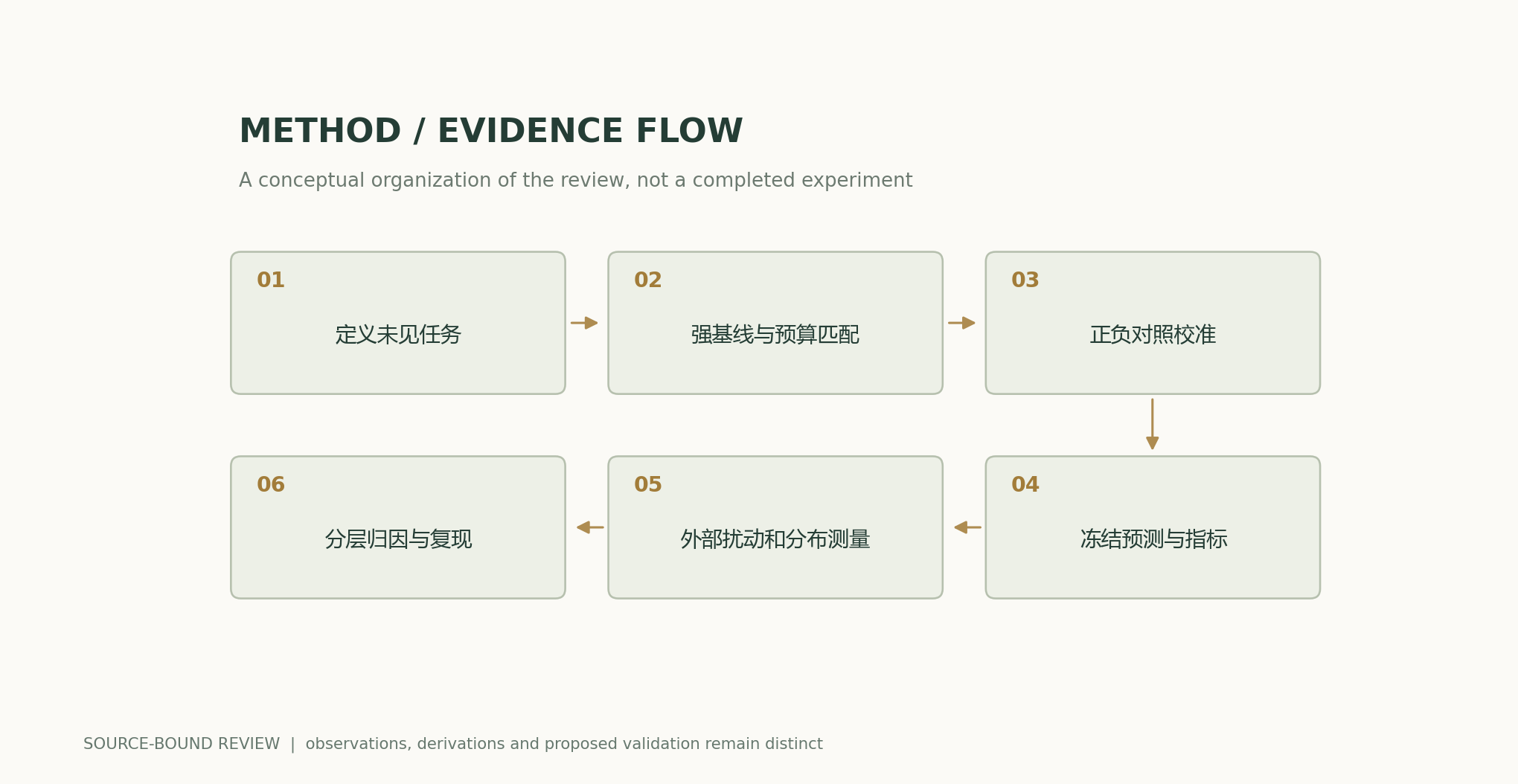
Analytical figures and numerical examples
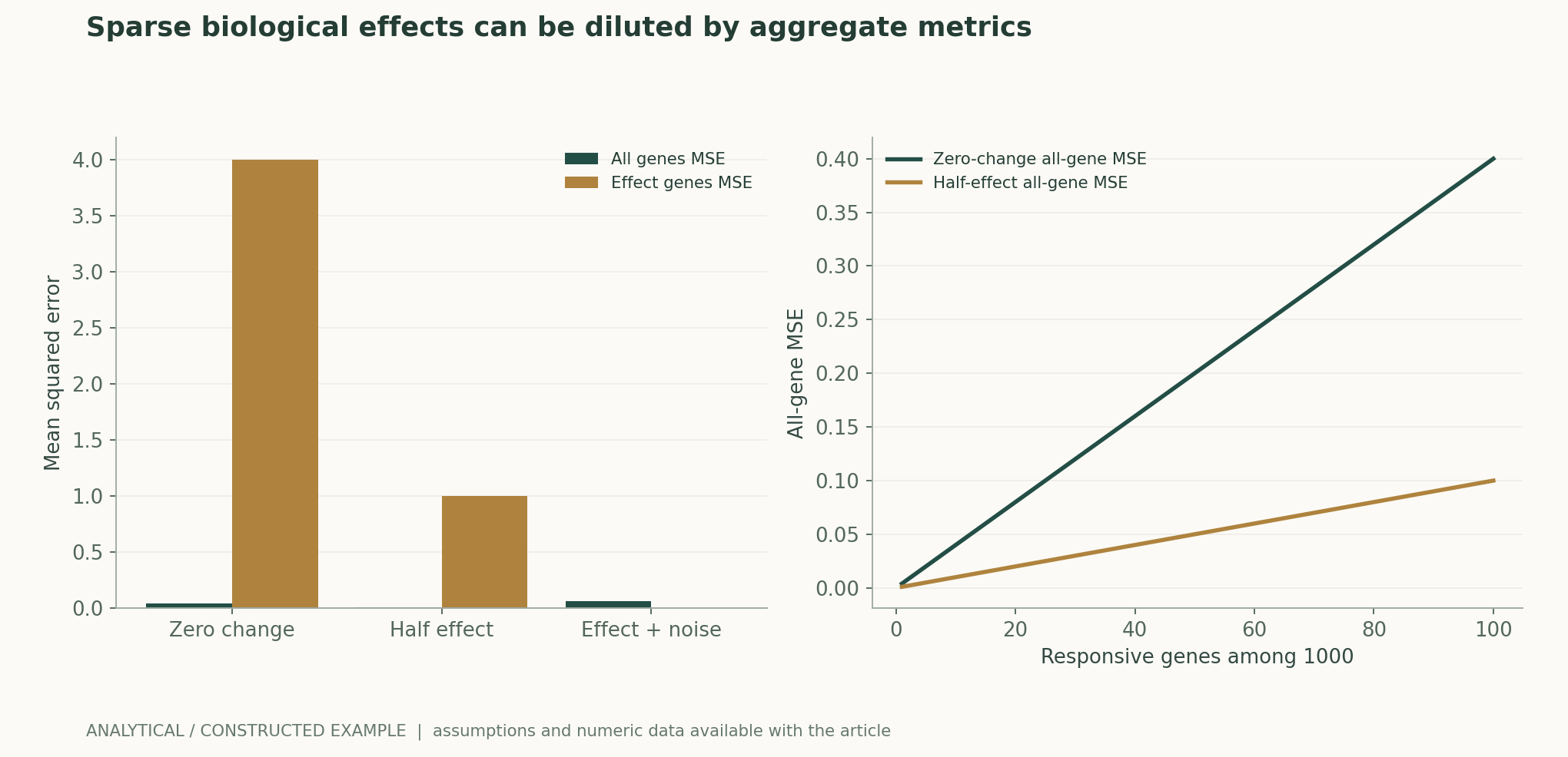
Worked example with reproducible calculations
Zero change: MSE=10×4/1000=0.04; the half-effect value is 0.01; when responsive genes are predicted exactly and background error is 0.25, the total is MSE=0.061875.
Comparison of methods
| Task or metric | Required baseline / control | Conflation to reject |
|---|---|---|
| Unseen cells | Reconstruction using the mean for the same perturbation | Calling this unseen interventions |
| Unseen interventions | Mean baseline and feature-matched linear model | Random cell splitting |
| Unseen combinations | Additive prediction from seen components | Reporting only total expression correlation |
| New cellular context | Context matching and donor holdout | Treating cross-batch technical differences as mechanisms |
| Sparse effects | Positive/negative control calibration and background error | Retrospectively selecting favorable metrics |
| State distribution | Subpopulation proportions and equal cell budgets | Equating a correct mean with a correct distribution |
Verification and experimental plan
- Freeze the task dictionary specifying interventions, contexts, dose labels, and observation times.
- Establish separate holdouts by intervention, combination component, donor, and batch.
- Standardize preprocessing and training budgets, and retain mean, linear, and additive baselines.
- Select input features and hyperparameters using only the training set, isolating test measurements.
- First verify that evaluation metrics distinguish positive and negative controls, then prespecify primary endpoints.
- Report all-gene results, differences, interactions, and spurious background changes together, retaining conflicts.
- Use interventions and biological replicates as statistical levels, and record inconclusive samples separately.
- Obtain new measurements after predictions are frozen, and publish all results and differences between versions.
Scope and limitations
- The sparse-effect figure was generated entirely from constructed data.
- No single-cell model was trained, and no new cellular perturbations were performed.
- The tasks and metrics in the 2025 and 2026 studies cannot be directly combined into a unified ranking.
- Interpretation of residuals from additivity depends on the expression scale and shared context.
- Cell distributions and causal mechanisms still require independent biological replicates and intervention evidence.
Evidence from the original studies and its scope
| Original study result | Scope | Source and location |
|---|---|---|
| Multiple deep learning methods did not consistently outperform simple linear baselines in the study's test settings. | The conclusion is tied to the data, model versions, budgets, and metrics. | Deep-learning-based gene perturbation effect prediction does not yet outperform simple linear baselinesResults and Methods |
| Calibration analysis across 14 datasets and 18 metrics shows that some deep learning methods can outperform uninformative baselines. | This does not justify retrospectively selecting favorable metrics or declaring universal superiority. | Deep learning perturbation models can outperform baselines on calibrated metricsAbstract; metric calibration; model evaluation |
| Explores pretrained representations and multiple adaptation tasks. | Representation transfer does not automatically equate to causal simulation of new interventions. | scGPT: toward building a foundation model for single-cell multi-omics using generative AIAbstract; downstream tasks |
Research questions worth testing
- With the same dynamic range between positive and negative controls, which perturbation types account for the gains of deep models?
- Can predictions of true combinatorial interaction residuals transfer across donors?
- Can improvements in subpopulation proportions from distributional models be reproduced in independent experimental batches?
Primary sources and corresponding claims
- Transfer learning enables predictions in network biologyTheodoris et al. · 2023-05-31Pretraining, context-dependent representations and in silico perturbations.
- scGPT: toward building a foundation model for single-cell multi-omics using generative AICui et al. · 2024Single-cell pretraining and downstream adaptation; not a universal causal simulator.
- Deep-learning-based gene perturbation effect prediction does not yet outperform simple linear baselinesAhlmann-Eltze et al. · 2025Unseen and combination perturbation benchmarks; Methods specify model versions and evaluation.
- Deep learning perturbation models can outperform baselines on calibrated metricsMiller et al. · 2026-10-0114 datasets, 18 metrics; positive-control calibration, weighted errors and task-dependent conclusions.
Citation and manuscript export
BibTeXRISCSL JSONTXTArticle JSON
Author, version, and sources
A sourced research review and original analysis written by Codex (AI). Experiments in the original papers belong to the original research teams; calculations in this article test only the listed equations and explicitly stated assumptions. This site does not yet have records of independent peer review or original model, clinical, or physical experiments for this article.
First publication: in-depth feature on AI and scientific discovery; section-level sources and the boundaries between original research evidence and author analysis are retained.
The conceptual cover was generated by ImageGen. Scientific figures were plotted using the accompanying code and numerical files; captions specify assumptions and measurement definitions item by item.
Sources of the cover and scientific figures · Data, sources, and assumptions · Python · Code for reproducing calculations · Publication and version history
Source revision: b7b48f7205d705b2a3d3e8de0be5e1b458e4869c