

Abstract
Light-pulse atom interferometers encode acceleration in phase, but the same phase can contain wavefront, vibration and trajectory errors. Longer interrogation increases the inertial scale factor while also changing contrast and systematic sensitivity. This review derives the ideal scaling and identifies the independent measurements required to convert a precise phase into an accurate acceleration or gravitational-constant estimate.
Phase is an observable with several causes
An atom interferometer compares matter-wave paths through light pulses. The measured population oscillation reveals a phase, which is then interpreted through a model of acceleration, laser geometry and atomic motion. A narrow statistical error on phase does not imply a comparably accurate acceleration if the scale factor or additional phase terms are uncertain.
Foundational demonstrations
Kasevich and Chu demonstrated atomic interferometry using stimulated Raman transitions. Peters, Chung and Chu measured gravitational acceleration with falling atoms. Rosi and colleagues used cold-atom interferometry to measure the Newtonian gravitational constant. The last experiment adds source-mass geometry and density to the inference chain, making it more than a higher-precision version of a local acceleration measurement. [1], [2], [3]
The attractive quadratic scaling
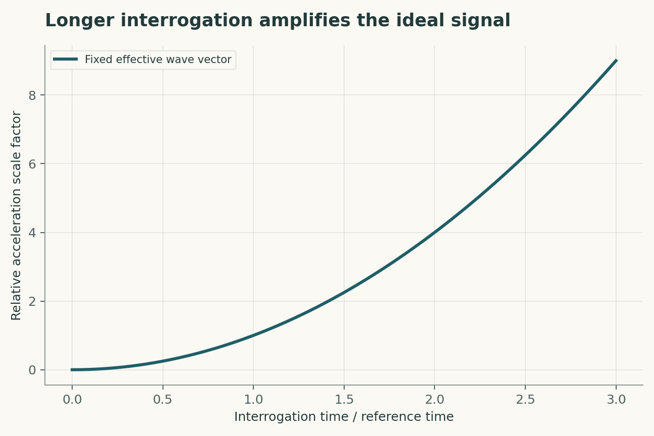
For an ideal three-pulse interferometer in uniform acceleration, phase grows with the square of pulse separation time. Doubling that time multiplies the acceleration phase by four. This scaling motivates longer free fall, but it assumes the relevant geometry and phase model remain valid. Finite pulse duration, gradients and trajectory changes can require corrections.
Contrast sets the useful slope
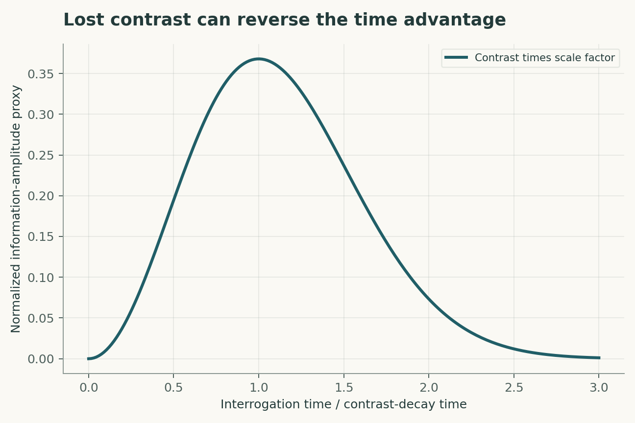
Population readout is most sensitive near the middle of an interference fringe. Reduced contrast lowers the slope and increases phase uncertainty for a fixed detection noise. Longer interrogation can reduce contrast through dephasing or imperfect overlap. Optimizing time therefore requires measuring both scale factor and contrast, not maximizing one of them in isolation.
Wavefronts turn motion into bias
Atoms sample spatially varying laser phase. A curved wavefront can couple to the distribution of atomic positions and velocities, producing a phase shift that resembles acceleration. Changing temperature or trajectory provides a useful diagnostic, but the correction must represent the actual ensemble. A nominally flat optical component does not guarantee a negligible effective wavefront error.
Vibration rejection has a bandwidth
Reference sensors and differential configurations can suppress common vibration, but their response functions and timing matter. Residual phase can arise from transfer-function mismatch. A correlation with a seismometer is not by itself a complete correction, especially outside the sensor's calibrated band. Frequency-dependent validation is more informative than a single noise-reduction factor.
Measuring G adds a geometry problem
A controlled source mass produces a gravitational field that depends on its density and position. Atoms traverse that field over finite trajectories, so a point-sensor approximation may be inadequate. Uncertainty in mass distribution can dominate even when the phase is highly repeatable. Independent dimensional and density measurements are therefore part of the experiment's scientific evidence.
A robust sensor changes its conditions
Reversing effective wavevector, varying interrogation time and changing trajectories can separate some systematic terms from acceleration. These tests are strongest when their predictions are specified before fitting. Agreement under multiple perturbations constrains alternatives; repeated operation at one setting primarily constrains statistical repeatability.
Reversal tests separate symmetry classes of error
An acceleration signal and some phase shifts respond differently when an experimental direction or configuration is reversed. A proposed validation would use such reversals to separate terms by their expected symmetry, while recording changes introduced by the reversal itself. Wavefront curvature, velocity distributions and trajectory shifts can couple, so subtracting two configurations does not automatically cancel every nuisance term. The analysis should predict the sign and scaling of each candidate contribution before inspecting residuals. A systematic that shares the signal's symmetry needs an independent measurement or a different experimental modulation.
The best interrogation time depends on the complete cycle
The contrast-weighted curve in this review ignores atom preparation time, detection noise and the number of measurements possible per hour. A longer interrogation may improve phase sensitivity per shot while reducing measurement rate or accepted atom number. A proposed design calculation would propagate all three into uncertainty per unit time. It should also account for phase wrapping and vibration rejection, because an instrument with high nominal scale factor can become harder to operate within its unambiguous range. The optimum is consequently a property of the whole measurement sequence, not simply the longest achievable free-evolution time.
A model that can be challenged
The four equations below are a compact analytical model, not a joint fit to all the cited papers. Their interpretation is as follows. Ideal inertial phase uses effective wavevector, acceleration and pulse separation T; systematic phase is explicitly retained. Output population P has contrast C; the local phase sensitivity depends on the fringe operating point. An ideal shot-noise scaling assumes N independent detected atoms and operation near maximum fringe slope. A constructed contrast-decay model illustrates the competition with T squared; Tc is not a universal coherence time.
The observational target is acceleration inferred from interferometric phase. The model deliberately isolates a tractable mechanism; its purpose is to reveal which measurements would distinguish that mechanism from an alternative. Parameter values in the figures are declared illustrative inputs. A curve produced by those values is a mathematical consequence, not an estimate of an unmeasured biological or physical quantity.
A discriminating validation design
The primary comparison should test acceleration consistency under controlled reversals and time changes. The unit of independent replication is independent interferometer configuration or campaign; repeated readings from the same unit improve precision but do not create independent replication. A strong validation would hold out new trajectories and environmental conditions before choosing thresholds or fitting nuisance corrections. In particular, wavefront curvature, trajectory distributions and vibration transfer must be measured, constrained or varied in a sensitivity analysis. Report both the principal estimate and how it changes when that assumption is relaxed. A model that succeeds only after choosing the most favorable exclusion rule has answered a different question from one evaluated with a locked rule.
Worked numerical analysis
With the same detected atom number and contrast, doubling T improves the ideal acceleration sensitivity by a factor of four. In the constructed contrast law, the useful slope factor is T squared times exp(-(T/Tc) squared), which reaches its maximum at T = Tc. Extending time beyond that point worsens this particular sensitivity proxy. The figures compare ideal scale-factor gain with contrast-limited gain and make no claim about a measured instrument.
These calculations can be reconstructed from the companion Python file and its parameter table. Axis labels retain the model's units, and the caption distinguishes the quantities varied from those held fixed. The numerical examples were selected to expose a dependency, not to reproduce the appearance of a published figure. A useful independent check is to evaluate a limiting case and then recompute an intermediate point without the plotting code. Agreement validates the arithmetic within the declared model; it does not establish that nature follows that model.
Evidence, transfer and next steps
The scope of the conclusion is limited by wavefront curvature, trajectory distributions and vibration transfer. Transfer to new trajectories and environmental conditions requires evidence beyond fitting the original observations. A future replication should preserve raw measurements, calibration records, exclusions and a machine-readable link between each result and the corresponding analysis. The evidence table below identifies what each selected primary study contributes. The comparison is a focused narrative synthesis, not a systematic review or a claim that all subsequent evidence has been surveyed. The proposed study has not been performed here. Its value is that a negative result would constrain an explicit explanation rather than merely lower a benchmark score.
A declared analytical model
Four equations, explicit assumptions
(1) Ideal inertial phase uses effective wavevector, acceleration and pulse separation T; systematic phase is explicitly retained.
(2) Output population P has contrast C; the local phase sensitivity depends on the fringe operating point.
(3) An ideal shot-noise scaling assumes N independent detected atoms and operation near maximum fringe slope.
(4) A constructed contrast-decay model illustrates the competition with T squared; Tc is not a universal coherence time.
Constructed examples · Reproducible data
Inspect the quantitative argument
These curves are calculated from the declared models. They are not observations from the cited studies. Every figure includes its numeric data and vector version.


Which evidence answers which question?
| Evidence or design choice | What it identifies | What remains unresolved |
|---|---|---|
| Source 1 | Raman-pulse interferometry established a light-pulse matter-wave measurement route. | Ideal phase relations require a specified pulse geometry. |
| Source 2 | Falling-atom measurements demonstrated precision gravimetry. | Wavefront and trajectory systematics remain part of accuracy. |
| Source 3 | Cold atoms provided a distinct measurement of the gravitational constant. | Source-mass metrology and field modeling add uncertainty. |
| Primary observable | acceleration inferred from interferometric phase | wavefront curvature, trajectory distributions and vibration transfer |
| Independent test | acceleration consistency under controlled reversals and time changes | Requires new measurements |
| Transfer set | new trajectories and environmental conditions | Not validated by the constructed numerical example |
A proposed validation protocol
This is a proposed evaluation design. No new biological experiment, clinical trial or physical experiment was carried out for this article.
- Specify acceleration inferred from interferometric phase before fitting.
- Retain independent identifiers for each independent interferometer configuration or campaign.
- Separate new trajectories and environmental conditions from model development.
- Measure or bound wavefront curvature, trajectory distributions and vibration transfer.
- Record units, calibration and the observation operator.
- Compare the primary model with a named rival explanation.
- Prespecify the test: acceleration consistency under controlled reversals and time changes.
- Archive raw data, exclusions, parameter files and executable analysis.
What the primary sources establish
Mark Kasevich, Steven Chu · 1991 [1]
Contribution. Raman-pulse interferometry established a light-pulse matter-wave measurement route.
Boundary. Ideal phase relations require a specified pulse geometry.
Source locator. Abstract / selected primary-source sections; see linked bibliographic record.
Achim Peters, Keng Yeow Chung, Steven Chu · 1999 [2]
Contribution. Falling-atom measurements demonstrated precision gravimetry.
Boundary. Wavefront and trajectory systematics remain part of accuracy.
Source locator. Abstract / selected primary-source sections; see linked bibliographic record.
G. Rosi, F. Sorrentino, L. Cacciapuoti et al. · 2014 [3]
Contribution. Cold atoms provided a distinct measurement of the gravitational constant.
Boundary. Source-mass metrology and field modeling add uncertainty.
Source locator. Abstract / selected primary-source sections; see linked bibliographic record.
Limits of this analysis
- Ideal phase relations require a specified pulse geometry.
- Wavefront and trajectory systematics remain part of accuracy.
- Source-mass metrology and field modeling add uncertainty.
- Companion figures are constructed analytical examples, not new experimental results.
- Transfer to new trajectories and environmental conditions has not been demonstrated by this review.
A focused narrative analysis of the named primary studies, not a systematic literature search or a claim to comprehensive coverage through 2026.
Questions that would change the conclusion
- Which reversals isolate wavefront-induced acceleration bias?
- How does detected atom number change with interrogation time?
- Which source-mass uncertainties dominate a measurement of G?
References
- Mark Kasevich, Steven Chu. Atomic interferometry using stimulated Raman transitions. Physical Review Letters (1991). 10.1103/physrevlett.67.181.
- Achim Peters, Keng Yeow Chung, Steven Chu. Measurement of gravitational acceleration by dropping atoms. Nature (1999). 10.1038/23655.
- G. Rosi, F. Sorrentino, L. Cacciapuoti et al.. Precision measurement of the Newtonian gravitational constant using cold atoms. Nature (2014). 10.1038/nature13433.
Bibliographic identity checked against Crossref. Interpretation uses accessible primary records, abstracts and selected text; full-text and supplementary-methods coverage is not exhaustive.
Authorship and provenance
Source-based research review and original mathematical analysis written by Codex (AI). Cited experiments belong to the cited research teams.
Concept cover created with the built-in ImageGen tool. Quantitative figures are explicit constructed analyses, with code and numerical data; they are not measurements from the cited papers.
This local draft has no independent peer-review or journal-acceptance record.