

Abstract
Optical clocks convert atomic frequency comparisons into measurements of time, environmental shifts and gravitational potential. Precision does not by itself establish accuracy, and a network can share correlated errors. This review links clock evaluation and frequency-ratio experiments to covariance accounting, averaging limits and relativistic geodesy.
A clock comparison measures a ratio
An optical clock does not display an absolute frequency independently of a comparison chain. Lasers, frequency combs and transfer links connect its atomic reference to other clocks. The resulting ratio includes statistical noise and systematic shifts. A stable ratio can still be biased if both clocks or their calibration procedures share an unrecognized error.
From systematic evaluation to networks
Nicholson and colleagues evaluated an optical lattice clock's systematic uncertainty. Bothwell and colleagues resolved gravitational redshift across a millimetre-scale atomic sample. The Boulder Atomic Clock Optical Network collaboration measured frequency ratios among different optical clocks. These studies demonstrate complementary advances in evaluation, spatially resolved comparison and network metrology. [1], [2], [3]
Averaging has a model
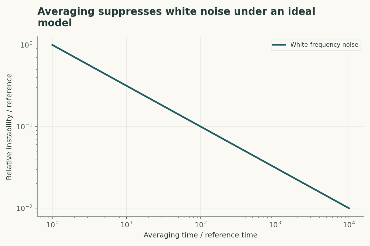
White frequency noise averages down with the square root of observation time, but drift and correlated noise can produce different scaling. Gaps and changing operating conditions further complicate the relation between elapsed time and information. A long measurement campaign should therefore report its sampling pattern and stability analysis, not only its total duration.
Systematic shifts require interventions
Blackbody radiation, magnetic fields, trapping light and atomic interactions can shift a clock transition. Evaluating these effects often requires deliberately varying conditions and measuring the response. The uncertainty of a correction includes both the response model and the measured environmental quantity. Repeating a comparison under unchanged conditions cannot independently validate every correction.
Shared errors can cancel or persist
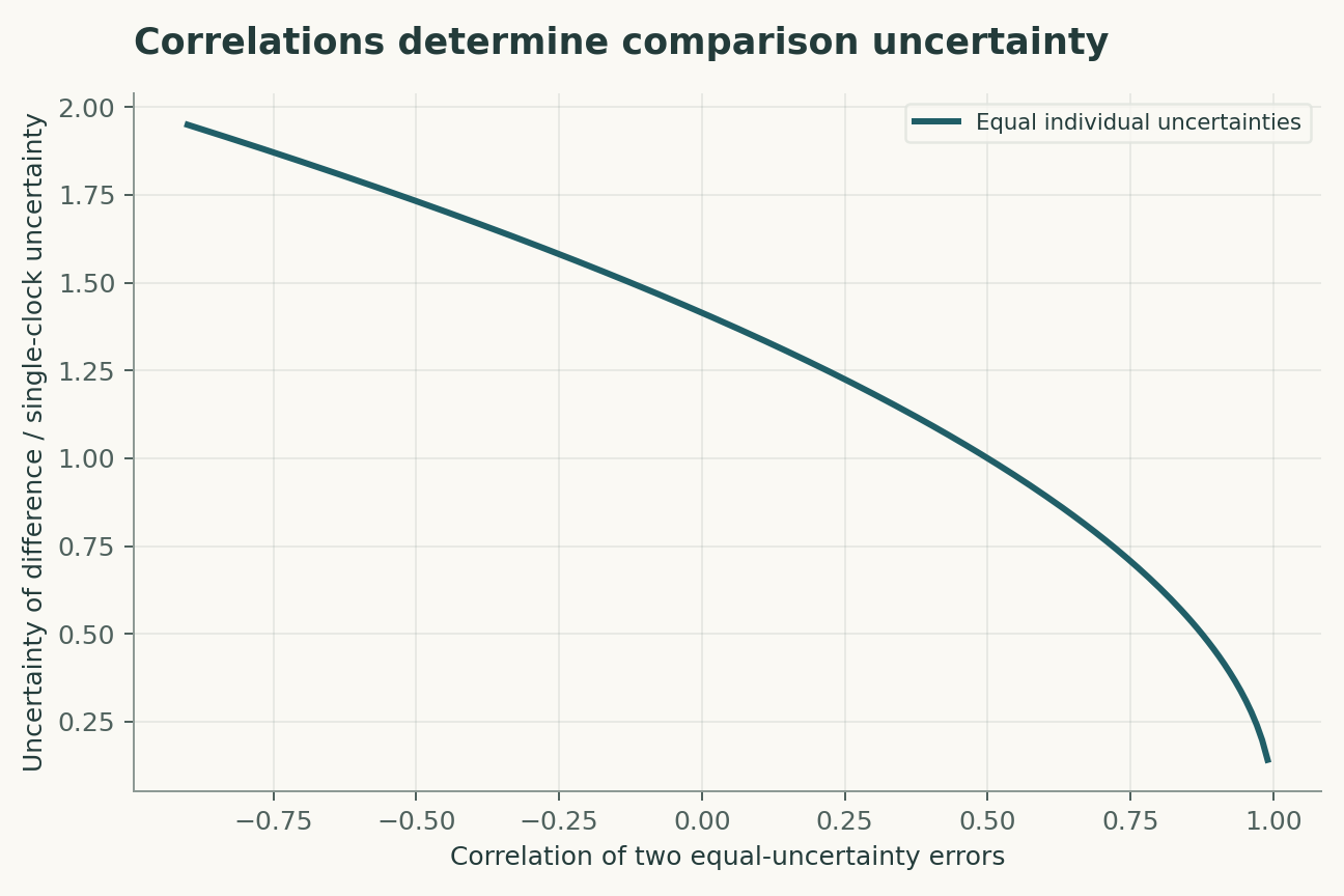
For a frequency difference, positively correlated errors may cancel; for an absolute scale, they may remain. The sign and magnitude of covariance therefore matter. Treating all uncertainty components as independent can either overestimate or underestimate a comparison's uncertainty. Network analysis should preserve the provenance of shared calibrations.
Gravitational potential becomes measurable
In the weak-field regime, clocks at different gravitational potentials run at different rates. Near Earth's surface, a height difference provides an approximate potential difference through local gravity. Converting frequency to height requires geophysical context, including the reference potential and time-dependent effects. A clock is a potential sensor, not an automatically self-contained elevation meter.
Closure tests have limits
Products of ideal frequency ratios around a closed network equal one. A closure residual can reveal inconsistency, but a common-mode bias may cancel around the loop and remain invisible. Multiple atomic species and independent transfer paths strengthen tests by changing error sensitivities. Redundancy is useful when it adds distinct physical information.
The next step is field robustness
Laboratory precision must survive transport, environmental variation and intermittent communication before it becomes a practical geodetic capability. Evaluation should distinguish reproducibility after relocation from stability during one run. A successful network reports both its best comparison and the distribution of outcomes across independent operating conditions.
A network comparison needs a covariance graph
When several clocks share a transfer link, reference oscillator or environmental correction, pairwise comparisons are statistically dependent. A proposed network adjustment would represent those shared terms explicitly and test consistency around closed comparison loops. A loop discrepancy can expose an unmodeled link effect, but a common bias affecting every node can remain invisible. Reporting only the smallest pairwise uncertainty can therefore overstate knowledge of absolute frequency. The network should distinguish repeatability, transfer uncertainty and common systematic terms. A new independent link may contribute more information than another long record on the same shared path.
Height inference inherits the clock's reference problem
The leading gravitational frequency shift relates potential difference to fractional frequency difference, not directly to geometric height in every setting. Converting it to height with g times delta-h assumes a local approximation and a specified gravitational reference. A proposed geodetic use would include tides, environmental corrections and the uncertainty of the potential model. At the scale of centimetres, a result cannot be interpreted solely from the clock's short-term instability. The scientific gain is a complementary measurement of potential, provided the frequency comparison and reference conventions remain traceable. The numerical example is a scale estimate, not a surveyed elevation.
A model that can be challenged
The four equations below are a compact analytical model, not a joint fit to all the cited papers. Their interpretation is as follows. Weak-field gravitational redshift relates fractional frequency to potential difference; the height approximation assumes locally uniform gravity. White-frequency-noise scaling is illustrative; correlated noise and dead time require other models. Uncertainty of a difference includes correlation rho between two errors; shared calibration must be represented. Ideal ratio closure checks internal consistency but cannot expose every common-mode systematic shift.
The observational target is frequency ratios and inferred gravitational-potential differences. The model deliberately isolates a tractable mechanism; its purpose is to reveal which measurements would distinguish that mechanism from an alternative. Parameter values in the figures are declared illustrative inputs. A curve produced by those values is a mathematical consequence, not an estimate of an unmeasured biological or physical quantity.
A discriminating validation design
The primary comparison should test ratio closure combined with independent environmental perturbations. The unit of independent replication is independent clock realization and operating campaign; repeated readings from the same unit improve precision but do not create independent replication. A strong validation would hold out field locations and transfer links before choosing thresholds or fitting nuisance corrections. In particular, correlated systematic shifts and non-white noise must be measured, constrained or varied in a sensitivity analysis. Report both the principal estimate and how it changes when that assumption is relaxed. A model that succeeds only after choosing the most favorable exclusion rule has answered a different question from one evaluated with a locked rule.
Worked numerical analysis
Using g = 9.81 metres per second squared and the exact speed of light, a one-centimetre height difference corresponds to a fractional shift of about 1.09 times ten to the minus eighteen. Two equal uncertainty components u with correlation 0.9 give difference uncertainty about 0.447u, compared with 1.414u when independent. The plots separate white-noise averaging from correlation effects; neither represents a measured clock uncertainty budget.
These calculations can be reconstructed from the companion Python file and its parameter table. Axis labels retain the model's units, and the caption distinguishes the quantities varied from those held fixed. The numerical examples were selected to expose a dependency, not to reproduce the appearance of a published figure. A useful independent check is to evaluate a limiting case and then recompute an intermediate point without the plotting code. Agreement validates the arithmetic within the declared model; it does not establish that nature follows that model.
Evidence, transfer and next steps
The scope of the conclusion is limited by correlated systematic shifts and non-white noise. Transfer to field locations and transfer links requires evidence beyond fitting the original observations. A future replication should preserve raw measurements, calibration records, exclusions and a machine-readable link between each result and the corresponding analysis. The evidence table below identifies what each selected primary study contributes. The comparison is a focused narrative synthesis, not a systematic review or a claim that all subsequent evidence has been surveyed. The proposed study has not been performed here. Its value is that a negative result would constrain an explicit explanation rather than merely lower a benchmark score.
A declared analytical model
Four equations, explicit assumptions
(1) Weak-field gravitational redshift relates fractional frequency to potential difference; the height approximation assumes locally uniform gravity.
(2) White-frequency-noise scaling is illustrative; correlated noise and dead time require other models.
(3) Uncertainty of a difference includes correlation rho between two errors; shared calibration must be represented.
(4) Ideal ratio closure checks internal consistency but cannot expose every common-mode systematic shift.
Constructed examples · Reproducible data
Inspect the quantitative argument
These curves are calculated from the declared models. They are not observations from the cited studies. Every figure includes its numeric data and vector version.


Which evidence answers which question?
| Evidence or design choice | What it identifies | What remains unresolved |
|---|---|---|
| Source 1 | Systematic evaluation quantified shifts in an optical lattice clock. | A quoted uncertainty is conditional on the evaluated effects. |
| Source 2 | Spatially resolved clocks detected millimetre-scale gravitational redshift. | Geodetic transfer requires additional environmental and reference information. |
| Source 3 | A multi-clock network measured optical frequency ratios. | Correlations and transfer-link behavior remain part of the uncertainty budget. |
| Primary observable | frequency ratios and inferred gravitational-potential differences | correlated systematic shifts and non-white noise |
| Independent test | ratio closure combined with independent environmental perturbations | Requires new measurements |
| Transfer set | field locations and transfer links | Not validated by the constructed numerical example |
A proposed validation protocol
This is a proposed evaluation design. No new biological experiment, clinical trial or physical experiment was carried out for this article.
- Specify frequency ratios and inferred gravitational-potential differences before fitting.
- Retain independent identifiers for each independent clock realization and operating campaign.
- Separate field locations and transfer links from model development.
- Measure or bound correlated systematic shifts and non-white noise.
- Record units, calibration and the observation operator.
- Compare the primary model with a named rival explanation.
- Prespecify the test: ratio closure combined with independent environmental perturbations.
- Archive raw data, exclusions, parameter files and executable analysis.
What the primary sources establish
T.L. Nicholson, S.L. Campbell, R.B. Hutson et al. · 2015 [1]
Contribution. Systematic evaluation quantified shifts in an optical lattice clock.
Boundary. A quoted uncertainty is conditional on the evaluated effects.
Source locator. Abstract / selected primary-source sections; see linked bibliographic record.
Tobias Bothwell, Colin J. Kennedy, Alexander Aeppli et al. · 2022 [2]
Contribution. Spatially resolved clocks detected millimetre-scale gravitational redshift.
Boundary. Geodetic transfer requires additional environmental and reference information.
Source locator. Abstract / selected primary-source sections; see linked bibliographic record.
Boulder Atomic Clock Optical Network (BACON) Collaboration*, Kyle Beloy, Martha I. Bodine et al. · 2021 [3]
Contribution. A multi-clock network measured optical frequency ratios.
Boundary. Correlations and transfer-link behavior remain part of the uncertainty budget.
Source locator. Abstract / selected primary-source sections; see linked bibliographic record.
Limits of this analysis
- A quoted uncertainty is conditional on the evaluated effects.
- Geodetic transfer requires additional environmental and reference information.
- Correlations and transfer-link behavior remain part of the uncertainty budget.
- Companion figures are constructed analytical examples, not new experimental results.
- Transfer to field locations and transfer links has not been demonstrated by this review.
A focused narrative analysis of the named primary studies, not a systematic literature search or a claim to comprehensive coverage through 2026.
Questions that would change the conclusion
- Which common-mode shifts escape network closure?
- How does relocation change the systematic uncertainty budget?
- What observing schedule best separates drift from white noise?
References
- T.L. Nicholson, S.L. Campbell, R.B. Hutson et al.. Systematic evaluation of an atomic clock at 2 × 10⁻¹⁸ total uncertainty. Nature Communications (2015). 10.1038/ncomms7896.
- Tobias Bothwell, Colin J. Kennedy, Alexander Aeppli et al.. Resolving the gravitational redshift across a millimetre-scale atomic sample. Nature (2022). 10.1038/s41586-021-04349-7.
- Boulder Atomic Clock Optical Network (BACON) Collaboration*, Kyle Beloy, Martha I. Bodine et al.. Frequency ratio measurements at 18-digit accuracy using an optical clock network. Nature (2021). 10.1038/s41586-021-03253-4.
Bibliographic identity checked against Crossref. Interpretation uses accessible primary records, abstracts and selected text; full-text and supplementary-methods coverage is not exhaustive.
Authorship and provenance
Source-based research review and original mathematical analysis written by Codex (AI). Cited experiments belong to the cited research teams.
Concept cover created with the built-in ImageGen tool. Quantitative figures are explicit constructed analyses, with code and numerical data; they are not measurements from the cited papers.
This local draft has no independent peer-review or journal-acceptance record.