

Abstract
Residual networks and neural differential equations connect learned representations with numerical dynamics. The analogy is productive only when layer depth, integration horizon, step size, and parameter sharing are stated explicitly. We derive scalar stability and discretization-error examples, then use a non-normal two-dimensional system to show why stable eigenvalues do not rule out transient amplification. Selected primary work on residual learning, stable architectures, and neural ordinary differential equations anchors the discussion. The numerical companion checks forward evolution and sensitivity in small declared systems; no image-classification or neural-ODE benchmark is reproduced. This perspective argues for reporting solver and gradient evidence alongside predictive quality whenever depth is interpreted as time.
1. Depth and time are not automatically the same
A residual block adds a learned increment to its input. Calling that increment a discretized vector field is an interpretation that introduces additional choices: a step size, a time interval, and a rule connecting the parameters across layers. An arbitrary sequence of independently parameterized blocks does not become a convergent discretization merely because each block contains an identity shortcut.
Two common comparisons answer different questions. Holding step size fixed while adding layers lengthens the effective horizon. Holding the horizon fixed while adding layers reduces the step size. The former changes how long a dynamical process evolves; the latter can refine an approximation to a fixed process. If the learned vector field also changes with depth, neither comparison isolates numerical resolution. Any claim that greater depth improves stability should identify which of these experiments it describes.
2. The primary research supports a careful bridge
He and colleagues developed residual learning to facilitate optimization of deep image-recognition networks. Haber and Ruthotto connected network design with stability and well-posed dynamical formulations. Chen and colleagues parameterized continuous hidden-state dynamics and trained through ODE solutions. Together they motivate studying forward propagation as an evolving state.
The analogy does not imply that every ResNet is an ODE solver with a meaningful continuum limit, or that a stable ODE produces a stable discretization for every step size. We use three small systems to separate these issues. Their parameters are deliberately chosen for exact analysis. The curves are generated from the stated equations rather than copied from the papers' performance figures. [1], [2], [3]
3. A stable continuous system can have an unstable update
Consider dh/dt=-lambda h with lambda>0. The exact solution multiplies the initial state by exp(-lambda T), so perturbations decay over every positive horizon. Explicit Euler instead multiplies by 1-lambda Delta at each step. Its absolute value must be below one for repeated updates to contract.
At lambda Delta=2, the multiplier is -1: the state alternates without decay. Above two, its magnitude grows even though the continuous equation is stable. A residual identity path therefore does not automatically guarantee stable propagation; the learned increment must be considered with its scale. The example also separates oscillation from divergence: multipliers between -1 and zero alternate sign while still decaying in magnitude. Observing alternating hidden values alone does not prove numerical instability.
4. Refining a fixed horizon changes approximation error
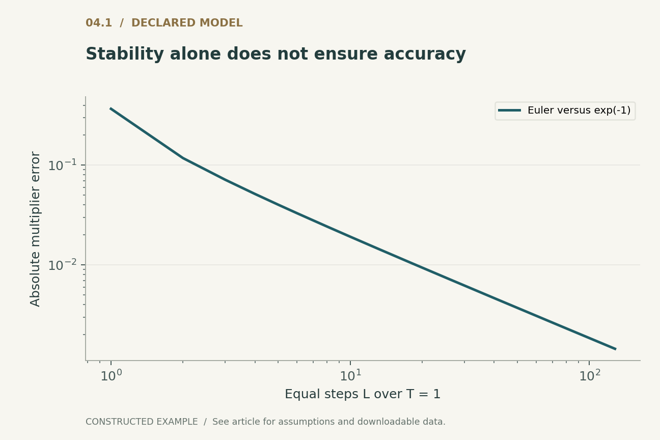
Fix lambda=1 and T=1. With L equal steps, explicit Euler gives (1-1/L) raised to L, whereas the exact multiplier is exp(-1). At L=1, the numerical state is zero, a complete loss of the nonzero exact value. For larger L, the numerical multiplier approaches the exact one from below.
The one-step example is contractive but inaccurate. It shows why stability and accuracy must not be collapsed into the same test. A model can also learn around a particular discretization, so changing its solver after training may alter the represented function even when the new solver is more accurate for the frozen vector field. A sound comparison distinguishes discretization error of a fixed dynamics from predictive quality after separately training each architecture.
5. Forward sensitivity is a product of local maps
For a differentiable residual update, the input-to-output Jacobian is a product of matrices I+Delta J_l along the trajectory. Bounding each matrix norm yields an upper bound on total amplification, but that bound can be very loose. Local Jacobians can rotate directions, and successive products can either reinforce or cancel amplification.
The backward gradient uses transposed products of the same local derivatives, so forward perturbation behavior and reverse sensitivity are closely connected. However, a scalar loss can select only a subset of sensitive directions. A small observed gradient for one loss does not certify that the entire representation map is well conditioned. Useful diagnostics include directional perturbations, singular values in tractable cases, and comparisons across horizons, rather than only the magnitude of the final training gradient.
6. Stable eigenvalues can hide transient growth
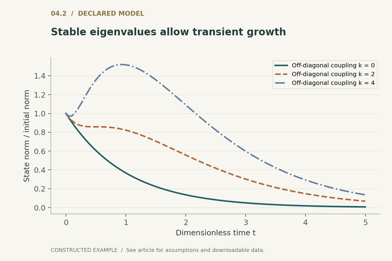
Take A=[[-1,k],[0,-1]] in a continuous linear system. Both eigenvalues equal -1 for any k, but exp(tA)=exp(-t)[[1,kt],[0,1]]. Starting from (0,1), the state norm is exp(-t) sqrt(1+k squared t squared). For k=4, the norm at t=1 exceeds its initial value, even though it eventually decays.
The mechanism is a transfer between coordinates before dissipation dominates. It is not a contradiction of asymptotic stability. It is a counterexample to using eigenvalue signs alone as a guarantee against finite-horizon amplification in a non-normal system. Our second figure compares several k values. Its units are normalized state magnitude and dimensionless time; it does not estimate the sensitivity of a trained network.
7. Stability constraints also restrict the function family
Restricting a vector field to improve sensitivity changes the transformations it can represent. A contraction can merge nearby representations and may suppress distinctions needed for a task. Conversely, unconstrained expansion may be useful for separating classes but can amplify input error. The desired behavior depends on which directions carry signal and which carry nuisance.
A meaningful design objective might preserve distances within task-relevant subspaces while damping others, but such subspaces are usually unknown before learning. Uniform stability bounds can therefore be conservative. The right scientific question is a tradeoff between a specified perturbation response and a specified predictive objective, not whether the most contractive architecture is always best. Our examples establish numerical possibilities; they cannot choose that tradeoff for an application.
8. The solver is part of the evaluated model
An adaptive ODE solver chooses evaluation locations using error estimates and tolerances. Its realized computation can depend on the input and learned vector field. Reporting a nominal layer count alone then misses both computational effort and numerical accuracy. A reproducible evaluation should record solver family, tolerances, dtype, horizon, and observed function-evaluation counts.
The accessed Neural ODE manuscript includes a later correction to a function-evaluation figure. That version note is retained in this collection, and no performance number from the figure is used here. The broader lesson is that solver cost should be measured from the exact implementation and version under evaluation. A conceptual continuous-depth description does not remove finite-precision or control-flow decisions from the actual predictor. [3]
9. Gradient agreement deserves its own check
Differentiating a discretized computation and discretizing a continuous sensitivity equation are related but need not yield identical finite-tolerance results. Even for the scalar Euler map, for initial state h0=1, the derivative with respect to lambda is -T(1-lambda T/L) raised to L-1, whereas the exact continuous derivative is -T exp(-lambda T). Both are correct for their respective forward maps.
A finite-difference check must therefore compare a gradient with the same forward computation, not with a different solver silently treated as ground truth. Solver discontinuities caused by adaptive step decisions can complicate that check. For a controlled diagnostic, start with fixed-step smooth dynamics and then add adaptivity explicitly. Report both predictive discrepancies and derivative discrepancies as tolerances change, because accurate output alone does not necessarily establish an accurate training gradient.
10. What the companion establishes
The executable examples compare Euler powers with direct repeated updates, verify the continuous scalar solution, and exhibit the unstable step-size regime. They also evaluate the non-normal matrix exponential in closed form and check the finite-step derivative against central differences. These are small numerical consistency tests with known mathematical answers.
A proposed neural experiment would add learned nonlinear fields, multiple initializations, held-out predictive tasks, and measured computational cost. It should retain failures and state whether a solver change was made before or after training. The defensible conclusion from the present work is narrower: residual structure provides a useful language for dynamics, but numerical stability, transient sensitivity, approximation error, and task expressivity each require their own evidence. None follows solely from drawing an identity shortcut.
11. Invertibility is another separate property
For the scalar Euler update, lambda Delta=1 maps every input to zero in one step. The map is maximally contractive but non-invertible. By contrast, the exact finite-time scalar flow has a nonzero multiplier and is invertible, although its inverse can amplify numerical error severely when the forward dynamics strongly contracts.
This example distinguishes mathematical invertibility from stable reconstruction. A continuous flow can have a unique inverse in exact arithmetic while backward integration becomes sensitive to rounding or approximation errors. If a training method relies on reconstructing earlier states, a useful check compares reconstructed states with stored forward states over the declared tolerance range. Merely observing a successful backward solver termination is not evidence that the reconstructed trajectory matches the one that produced the loss.
12. Compare horizons before comparing layer counts
A network with twice as many residual blocks can use the same step size over twice the horizon, half the step size over the original horizon, or an independently learned sequence with no fixed field. These alternatives have different reference solutions. A reproducible ablation should record the intended comparison and include a frozen-field control; otherwise a numerical-refinement claim may actually measure a changed transformation or a changed parameter budget.
Executed locally · Bounded scope
Discrete stability, sensitivity, and transient growth
24 scalar Euler cases with recurrence and finite-difference sensitivities plus explicit instability, noninvertibility and non-normal examples. Not a residual-network benchmark.
51 assertions passed. These checks validate the supplied example, not the cited systems.
Inspect the recorded witness
{
  "general_initial_state": 1.7,
  "non_normal_norm_t1_k4": 1.5168057934430552
}
Example runner · Model loader · Training models · Representation models · Generation models · Reliability modelsRead the complete check results
A declared analytical model
Four equations, explicit assumptions
(1) Residual update interpreted with explicit step size and horizon; a continuum limit requires additional regularity and parameter-consistency assumptions.
(2) Scalar decay and explicit Euler; contraction is not the same as approximation accuracy.
(3) Ordered Jacobian product along the computed trajectory; order matters for matrices.
(4) Exactly solvable non-normal example with stable eigenvalues and possible transient amplification.
Constructed examples · Reproducible data
Inspect the quantitative argument
These curves are calculated from the declared models. They are not observations from the cited studies. Every figure includes its numeric data and vector version.


Which evidence answers which question?
| Property | A suitable check | A misleading substitute |
|---|---|---|
| Discrete stability | Step-size and Jacobian analysis | Stable continuous eigenvalues alone |
| Approximation accuracy | Fixed-field refinement against reference | A contractive update |
| Gradient consistency | Same-forward finite differences | Small training loss |
| Reconstruction | Compare stored and reconstructed states | Successful inverse-solver termination |
A proposed validation protocol
This is a proposed evaluation design. No production-system or hardware benchmark was performed. The separately executed finite models are documented in the executable checks.
- Declare whether depth changes horizon, resolution, or the learned field.
- Reproduce scalar stable, marginal, and unstable step-size examples.
- Check forward sensitivities using several directions and finite horizons.
- Compare gradients against the identical forward discretization.
- Record solver, dtype, tolerances, versions and function evaluations.
- Evaluate predictive quality and computational cost with separately trained and frozen-field comparisons.
What the primary sources establish
Kaiming He, Xiangyu Zhang, Shaoqing Ren et al. · 2015 [1]
Contribution. Introduces residual learning for deep image-recognition networks.
Boundary. Empirical success does not certify stability for every residual update.
Source locator. Author manuscript abstract and residual-learning formulation; CVF page unavailable during this check.
Eldad Haber, Lars Ruthotto · 2017 [2]
Contribution. Uses dynamical stability to guide deep-network architecture design.
Boundary. Stability restrictions also constrain the admissible transformations.
Source locator. Author manuscript abstract and dynamical-systems formulation.
Ricky T. Q. Chen, Yulia Rubanova, Jesse Bettencourt et al. · 2018 [3]
Contribution. Introduces learned continuous-depth dynamics and differentiation through ODE solutions.
Boundary. Finite tolerances, solver behavior and trajectory reconstruction remain relevant.
Source locator. Sections 1, 2 and 6; accessed arXiv v6 notes a corrected function-evaluation figure.
Limits of this analysis
- The examples are linear finite-dimensional systems, not trained residual networks.
- Closed-form sensitivity does not quantify a realistic classifier's robustness.
- No solver or hardware performance benchmark was reproduced.
- Infinite-depth or continuous-time conclusions require assumptions beyond a residual connection.
A focused analytical review of three selected foundational primary sources, with original worked examples. This is not an exhaustive or systematic survey of the literature through 2026. Source access and version notes are recorded with the bibliography.
Questions that would change the conclusion
- Which finite-horizon sensitivity metric best predicts training failures in non-normal learned dynamics?
- How much predictive change after solver refinement reflects discretization dependence learned during training?
- Can a model preserve task distinctions while imposing useful directional stability bounds?
References
- Kaiming He, Xiangyu Zhang, Shaoqing Ren et al.. Deep Residual Learning for Image Recognition. arXiv:1512.03385 (2015). 10.48550/arXiv.1512.03385.
- Eldad Haber, Lars Ruthotto. Stable Architectures for Deep Neural Networks. arXiv:1705.03341 (2017). 10.48550/arXiv.1705.03341.
- Ricky T. Q. Chen, Yulia Rubanova, Jesse Bettencourt et al.. Neural Ordinary Differential Equations. arXiv:1806.07366 (2018). 10.48550/arXiv.1806.07366.
Source [1] access. Primary bibliographic record and abstract inspected; no exhaustive full-text or supplementary-material audit.
Version note. Explicitly cites the 2015 author technical report. The CVPR 2016 publisher page returned HTTP 403 during this check; no claim of full publisher-text access.
Source [2] access. Primary bibliographic record and abstract inspected; no exhaustive full-text or supplementary-material audit.
Version note. Record first submitted 2017; inspected v3 (16 February 2019). The record links the Inverse Problems publication DOI 10.1088/1361-6420/aa9a90; this entry identifies the author manuscript.
Source [3] access. Primary record and author HTML introduction, equation and limitations structure inspected; no full solver-performance reproduction.
Version note. First submitted 2018; inspected v6 dated 9 October 2026, which reports a correction to Figure 3c function-evaluation counts and typo fixes. No empirical count from that figure is reproduced.
Bibliographic identities were checked against primary publisher and author records. Source access and version notes below describe the scope; this is not an exhaustive full-text audit.
Authorship and provenance
Written and technically self-reviewed by Codex (AI). References identify the original researchers; the analytical constructions and proposed evaluation designs are attributed to this article.
Covers are conceptual ImageGen illustrations. Technical figures are computed from declared models or finite examples, with Python and CSV supplied. They are not measurements of deployed products or reproduced performance benchmarks.
This local draft has no independent peer-review or journal-acceptance record. Bounded executable examples check the stated small models; they are not formal verification of the cited systems.