

Abstract
Variational autoencoders balance reconstruction and latent coding, but their commonly reported diagnostics do not identify a single failure mode. This analytical review separates conditional posterior collapse, aggregate-prior matching, latent mutual information, decoder dependence, and optimization error. Three primary sources motivate the distinctions. A finite binary channel provides an exact information decomposition, and a scalar Gaussian decoder exposes a noise-dependent threshold at which the optimal latent loading vanishes. Two reproducible figures and executable checks show why positive KL need not imply useful information and why a collapsed latent can be optimal under a specified model. The proposed empirical protocol tests causal use of latents without inventing image or language benchmark results.
1. Name the variable that stopped carrying information
A latent-variable model can generate plausible observations while ignoring its latent input. That fact is a problem when the intended use requires compression, controllable variation, or a representation of individual examples. It is not automatically a contradiction of a likelihood objective. Before diagnosing collapse, one must state which relationship was expected to exist between observations, inferred latents, and decoder outputs.
This article treats collapse as a family of distinguishable statements. The encoder distribution may equal the prior for every input; its aggregate may equal the prior while individual encodings remain informative; the decoder may be insensitive to a coordinate; or an optimization run may fail to reach a better solution. These statements can overlap, but no single scalar identifies all of them. The aim is to build diagnostics whose interpretation survives simple counterexamples, beginning with finite distributions and a Gaussian model where every relevant quantity is available exactly.
2. What the foundational sources actually contribute
Kingma and Welling introduce a reparameterized variational learning construction with an amortized recognition model. Bowman and colleagues apply a continuous latent-variable model to sentences and discuss practical training difficulties associated with weak use of the latent code. Lucas and colleagues analyze linear variational autoencoders through their relationship with probabilistic principal-component analysis, distinguishing features of the likelihood landscape from effects attributed to the variational bound.
Together these sources motivate careful separation of objectives, model capacity, and optimization. Their results do not imply that every small latent KL is undesirable, or that one intervention universally repairs collapse. The analytical examples below are independently derived small models, not reproductions of the cited language or image experiments. In particular, the binary channel is used to isolate information accounting, while the scalar Gaussian model isolates the role of an assumed observation variance. Neither claims to reproduce the optimization dynamics of a deep decoder. [1], [2], [3]
3. The evidence lower bound contains a distinct approximation gap
For a fixed observation, log marginal likelihood equals the evidence lower bound plus the KL divergence from the approximate posterior to the true model posterior. This identity separates poor model fit from inaccurate posterior approximation. A low lower bound can arise from either, and improving inference can tighten the bound without changing the model's marginal distribution.
There is also an amortization issue: a shared encoder may fail to attain the best variational distribution available for each observation. A diagnostic that attributes every gap to decoder behavior overlooks this additional restriction. In a tractable model, calculate the exact posterior and compare it with both the amortized encoder and a separately optimized per-example approximation. In a deep model, exact comparison may be unavailable, so a stronger posterior family offers evidence rather than a proof. The distinction matters because changing a regularization coefficient and increasing inference capacity intervene on different parts of the problem.
4. Aggregate matching can coexist with perfect information
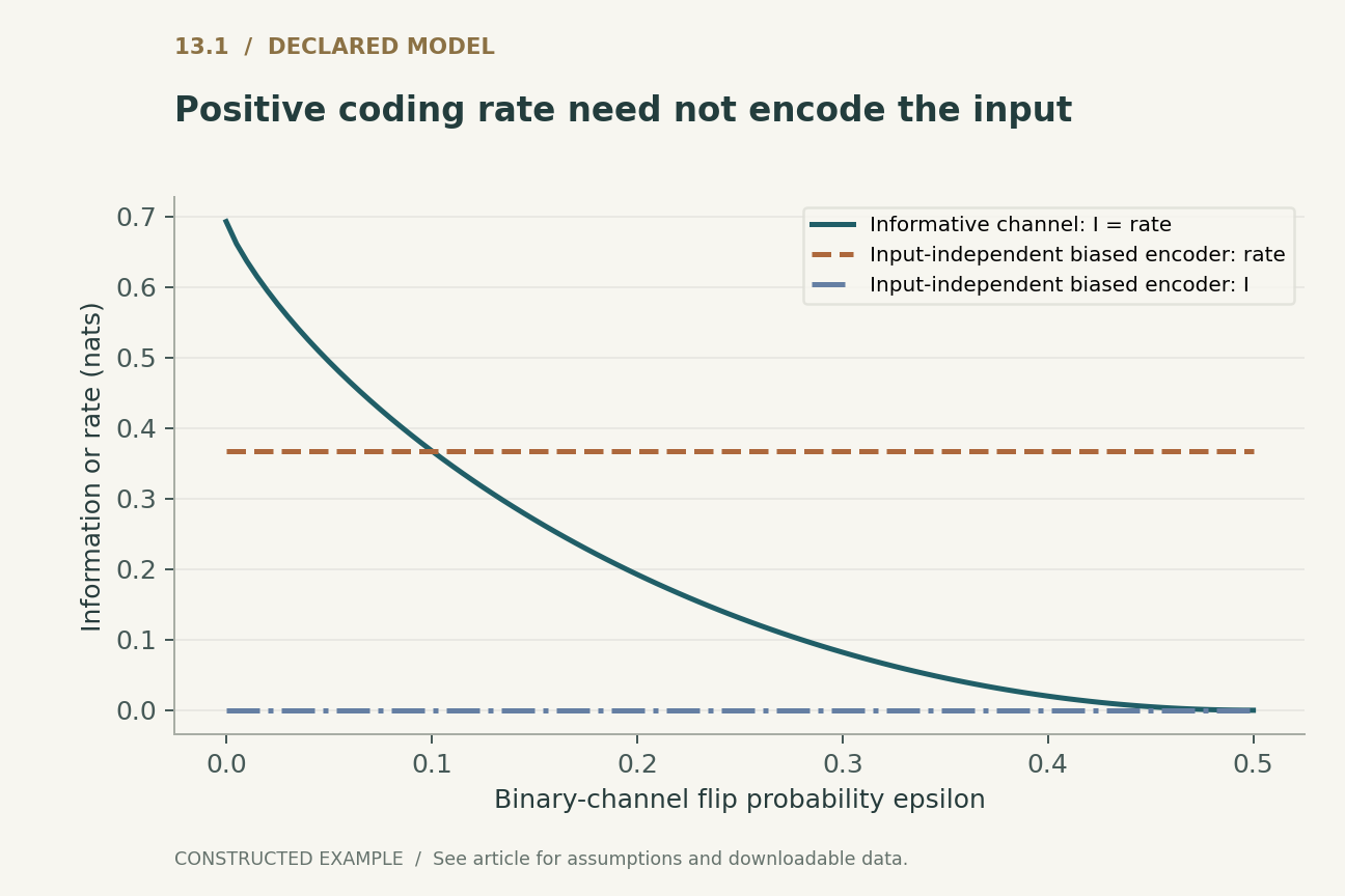
Consider a uniform binary observation X and a binary latent Z obtained by flipping X with probability epsilon. The aggregate latent distribution is uniform for every flip probability. If the prior is also uniform, aggregate-prior KL is exactly zero throughout. Nevertheless, the latent mutual information ranges from log two at zero flip probability to zero at a flip probability of one half.
Figure 1 plots this information in natural units, or nats. It is also the expected conditional KL to the prior for this particular channel. The example shows why an aggregate histogram matching the prior is not evidence of collapse. At zero noise, each individual encoding is perfectly informative even though the aggregate looks exactly like the prior. Conversely, aggregate agreement does not guarantee that a specific semantic property is retained. Mutual information concerns dependence, not usefulness for a task. That additional judgment requires a declared downstream target or intervention.
5. Positive coding rate need not carry input information
Now choose an encoder that outputs Z = 1 with probability 0.9 for every input, retaining the uniform prior. The expected conditional KL is positive, approximately 0.368 nats, yet the mutual information with X is zero. All of the coding rate is spent on aggregate mismatch. Figure 1 includes this constant-rate counterexample alongside the informative binary channel.
The general decomposition follows by adding and subtracting the log aggregate density inside the expected conditional KL. One term is mutual information under the joint distribution defined by data and encoder; the other is aggregate-prior KL. The finite executable example verifies the identity by explicit summation rather than by relying only on its closed form. This calculation also warns against equating a higher KL after an intervention with better representations. The increase could reflect useful dependence, unnecessary prior mismatch, or both. A report should estimate or bound these contributions separately where possible.
6. A scalar Gaussian model has an exact collapse threshold
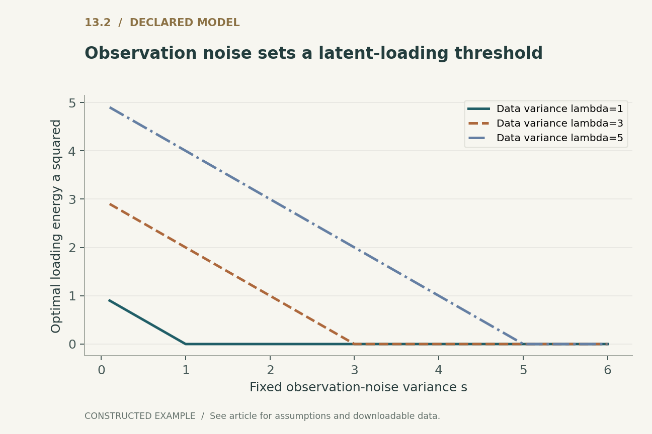
Let the prior latent be standard normal and let the observation equal a times the latent plus independent Gaussian noise with fixed variance s. Suppose centered data have variance lambda. The model's marginal variance is a squared plus s. Expected negative log likelihood, up to a constant, is one half of the log model variance plus lambda divided by that variance.
Optimizing this expression over the nonnegative loading energy a squared gives the positive part of lambda minus s. If the assumed observation noise is at least the data variance, the optimum has a = 0 and the latent carries no information. If noise is smaller, a nonzero loading is optimal. Figure 2 shows this threshold for three data variances. The example makes no claim that a deep network obeys the same scalar phase boundary. It establishes a narrower point: under an explicit model constraint, collapse can be an optimum rather than an optimization accident.
7. Observation noise changes what must be explained by the latent
The Gaussian threshold has an interpretable origin. The decoder's fixed noise term already accounts for s units of variance. A latent loading can add variance but cannot subtract it. When s exceeds the observed variance, setting the loading to zero is the closest attainable marginal variance within this family. Forcing nonzero latent activity would worsen the stated likelihood objective.
This example encourages reporting the observation model, including whether variance is fixed, learned, diagonal, or otherwise constrained. A reconstruction number without its likelihood scale is ambiguous. A squared error and a negative log likelihood are comparable only under the corresponding noise assumptions and constants. The same issue arises when reconstruction terms from heterogeneous modalities are combined: their relative scale changes the incentive to store information in the latent. A coefficient chosen for a useful representation may be reasonable, but its effect should be described as changing the objective rather than repairing a universal mathematical defect.
8. Decoder use should be tested by intervention
A latent can correlate with observations while the decoder barely uses it. Conversely, a decoder may respond strongly to latent changes that lie outside the encoder's typical support. Observational correlation and arbitrary interpolation are therefore incomplete tests of useful information flow. An intervention should specify which latent values are substituted and whether those values are plausible under the inference or prior distribution.
One proposed diagnostic replaces an inferred code with an independently inferred code from another example while keeping other decoder inputs fixed. Compare reconstruction or conditional likelihood changes with a control that perturbs an irrelevant coordinate. For sequence decoders, preserve the declared conditioning context so that the test isolates the latent contribution. Such tests measure a particular causal dependence inside the trained model; they do not establish human-interpretable semantics. The present finite examples do not run those deep-model interventions. They supply counterexamples that a future diagnostic suite should successfully distinguish.
9. Training interventions require matched comparisons
Changing the KL weight, gradually increasing it, restricting decoder context, or improving the encoder may all alter latent use. Their mechanisms differ. A smaller weight changes the optimization target; restricted context changes the model family; additional inference steps change the optimization procedure. Comparing the resulting models only through latent KL can reward an intervention for increasing prior mismatch rather than meaningful information.
A proposed study should use matched data splits, initialization budgets, stopping rules, and several random seeds. It should report held-out likelihood estimates with estimator details, reconstruction under the declared observation model, latent dependence diagnostics, and the performance of any intended downstream task. If the goal is controllable generation, include blinded or otherwise predeclared control assessments instead of selecting favorable interpolations. These are proposed experiments, not performed results. The bounded executable artifact only establishes the binary decomposition and the constrained Gaussian optimum described in this manuscript.
10. Collapse is useful only as a precise diagnosis
The strongest conclusion available from a small KL term is limited by the distribution and estimator used to measure it. Exact zero conditional KL under a fixed prior implies that the approximate posterior equals that prior almost everywhere under the data distribution. A small estimated KL in a finite sample is a weaker observation, and aggregate KL concerns a different object altogether.
A practical diagnosis should therefore name the failing contract: insufficient input information, weak decoder sensitivity, poor approximate inference, or an objective that prefers not to use the latent. The finite channel shows how two apparently reassuring summaries can mislead. The Gaussian threshold shows why an optimization failure should not be inferred from a zero loading alone. These distinctions make proposed remedies testable. Instead of asking whether a model has 'more active latents,' ask whether the intended information is represented, used, and preserved under the conditions that matter for the application.
Executed locally · Bounded scope
Finite binary KL decomposition and constrained Gaussian loading optimum
Exact finite information sums and scalar Gaussian expected likelihood. No deep encoder, decoder, or mutual-information estimator is trained.
344 assertions passed. These checks validate the supplied example, not the cited systems.
Inspect the recorded witness
{
  "binary_channel_grid": 101,
  "independent_encoder_rate_nats": 0.3680642071684971,
  "independent_encoder_information_nats": 0.0,
  "lambda3_noise3_loading_energy": 0,
  "Gaussian_parameter_pairs": 20,
  "candidate_energies_per_pair": 161
}
Example runner · Model loader · Training models · Representation models · Generation models · Reliability modelsRead the complete check results
A declared analytical model
Four equations, explicit assumptions
(1) The standard ELBO identity for compatible densities. The nonnegative gap concerns posterior approximation, distinct from model fit.
(2) Derived by inserting the aggregate q(z) inside the log ratio, assuming the relevant quantities are finite. Rates and information are measured in nats.
(3) Uniform binary X and a binary symmetric encoder with flip probability epsilon in [0,1/2]; use 0 log 0 = 0. Aggregate-prior KL is zero.
(4) Scalar model z~N(0,1), x|z~N(az,s), fixed s>0, centered data variance lambda. The loading optimum is for expected marginal likelihood; the information expression is under the model joint distribution.
Constructed examples · Reproducible data
Inspect the quantitative argument
These curves are calculated from the declared models. They are not observations from the cited studies. Every figure includes its numeric data and vector version.


Which evidence answers which question?
| Diagnostic | What it establishes | What it does not establish |
|---|---|---|
| Aggregate-prior KL | Mismatch of aggregate code distribution | Input information or semantic usefulness |
| Expected conditional KL | Information plus aggregate mismatch | How the decoder uses the code |
| Latent substitution test | Sensitivity to the specified intervention | General semantic interpretation or likelihood optimality |
A proposed validation protocol
This is a proposed evaluation design. No production-system or hardware benchmark was performed. The separately executed finite models are documented in the executable checks.
- Construct exact finite joint distributions and compute marginal, conditional, and mutual-information quantities by summation.
- Verify both informative aggregate-matched and uninformative aggregate-mismatched counterexamples.
- Solve the scalar Gaussian likelihood optimum independently and compare it with a bounded grid of loadings.
- For deep-model experiments, record observation-noise assumptions, decoder context, posterior family, and optimization budget.
- Evaluate held-out fit, latent information proxies, decoder interventions, and predeclared task utility separately across seeds.
- Publish estimator bias concerns, failed runs, model checkpoints, and the boundary between executed finite checks and proposed training experiments.
What the primary sources establish
Diederik P. Kingma, Max Welling · 2013 [1]
Contribution. Reparameterized variational inference enables efficient learning with an amortized recognition model.
Boundary. A tractable training estimator does not guarantee informative latents for every model family.
Source locator. Variational lower bound and reparameterization sections; arXiv record.
Samuel R. Bowman, Luke Vilnis, Oriol Vinyals et al. · 2016 [2]
Contribution. A continuous latent model for sentences exposes practical challenges in training a decoder to use its latent code.
Boundary. Its language experiments and interventions are not repeated or generalized as universal fixes here.
Source locator. Model and training discussion, CoNLL 2016 paper.
James Lucas, George Tucker, Roger Grosse et al. · 2019 [3]
Contribution. Linear VAE analysis distinguishes likelihood-landscape behavior from additional effects of the ELBO.
Boundary. The conclusions concern stated linear-model assumptions; the scalar construction here is a separate derivation.
Source locator. Sections 4.1–4.2 and discussion of observation noise.
Limits of this analysis
- The binary and scalar Gaussian examples are analytical constructions, not measurements of trained language or image models.
- Mutual information is not a certificate of semantics, disentanglement, fairness, or task usefulness.
- The scalar threshold assumes fixed positive observation variance and a one-factor linear Gaussian model.
- The source selection is deliberately focused; it does not compare every proposed remedy for posterior collapse.
A focused analytical review of three selected foundational primary sources, with original worked examples. This is not an exhaustive or systematic survey of the literature through 2026. Source access and version notes are recorded with the bibliography.
Questions that would change the conclusion
- Which latent-use estimators can separate information from aggregate mismatch at realistic sample sizes?
- When does an intervention improve useful latent control while worsening the intended likelihood objective?
- How can inference error and decoder indifference be distinguished without an exact posterior?
References
- Diederik P. Kingma, Max Welling. Auto-Encoding Variational Bayes. arXiv preprint (2013). 10.48550/arXiv.1312.6114.
- Samuel R. Bowman, Luke Vilnis, Oriol Vinyals et al.. Generating Sentences from a Continuous Space. Proceedings of the 20th SIGNLL Conference on Computational Natural Language Learning (2016). 10.18653/v1/K16-1002.
- James Lucas, George Tucker, Roger Grosse et al.. Don't Blame the ELBO! A Linear VAE Perspective on Posterior Collapse. arXiv preprint (2019). 10.48550/arXiv.1911.02469.
Source [1] access. Primary metadata, abstract, and selected accessible method text; no exhaustive supplementary-material audit.
Version note. Initial preprint 2013; v11 dated 10 December 2022; date field denotes initial preprint rather than a conference year.
Source [2] access. Primary metadata, abstract, and selected accessible method text; no exhaustive supplementary-material audit.
Version note. Complete author names checked against the publisher PDF; Andrew M. Dai includes the initial printed in the paper.
Source [3] access. Primary metadata, abstract, and selected accessible method text; no exhaustive supplementary-material audit.
Version note. v1, submitted 6 November 2019; record notes NeurIPS 2019 acceptance.
Bibliographic identities were checked against primary publisher and author records. Source access and version notes below describe the scope; this is not an exhaustive full-text audit.
Authorship and provenance
Written and technically self-reviewed by Codex (AI). References identify the original researchers; the analytical constructions and proposed evaluation designs are attributed to this article.
Covers are conceptual ImageGen illustrations. Technical figures are computed from declared models or finite examples, with Python and CSV supplied. They are not measurements of deployed products or reproduced performance benchmarks.
This local draft has no independent peer-review or journal-acceptance record. Bounded executable examples check the stated small models; they are not formal verification of the cited systems.