

Abstract
High predictive accuracy does not automatically answer the question, “What happens if a factor is changed?” This article distinguishes observational conditional distributions from interventional distributions, derives how confounding changes associations within explicit structural equations, and discusses the conditions for backdoor adjustment, representation identification, and distribution shift. The accompanying figures come from an exhaustively enumerable binary-confounder model whose variables and probabilities are fully disclosed; this is not a study of an actual population or policy effects.[1] Towards Causal Representation Learning[2] Invariant Risk Minimization[3] WILDS: A Benchmark of in-the-Wild Distribution Shifts
English abstract
Causal inference requires identification assumptions in addition to predictive accuracy. We distinguish observational conditioning from intervention and work through an explicit binary-confounder model. The calculated association and causal effect differ despite a fixed structural equation. No real treatment effect or policy recommendation is estimated; the example demonstrates assumptions and non-identification risks.
1. Prediction and intervention questions use different distributions
The observational distribution P(Y|X=x) describes the group in which X takes a particular value in data that have already occurred; the interventional distribution P(Y|do(X=x)) describes the system's outcomes after X is externally set. The two may differ because of common causes. Causal graphs and structural equations make assumptions explicit, but a graph itself is not a truth automatically obtained from a high-performing predictor. Variable meanings, temporal order, omitted factors, and admissible interventions must be specified; in particular, statistically controlling for arbitrary variables must not be assumed to always eliminate bias.[1] Towards Causal Representation Learning
2. A binary-confounder model reveals the difference exactly
Let U take 0 or 1 with equal probability, with P(X=1|U=1)=0.8 and P(X=1|U=0)=0.2, and let the outcome be Y=2X+5U. Among those observed with X=1, the proportion with U=1 is 0.8, whereas among those with X=0 it is 0.2; thus, the observational mean difference is 2+5×0.6=5. When intervening on X, the distribution of U remains unchanged, and the mean difference is only 2. There is no sampling error here: the discrepancy arises from the generating mechanism. With real data, one must also establish whether these conditions are credible.[1] Towards Causal Representation Learning
3. Backdoor adjustment depends on testable and untestable conditions
If U satisfies appropriate adjustment conditions, the interventional mean can be calculated from conditional means weighted by the population distribution P(U). Consistency, positive support within the relevant strata, and adequate measurement quality are also required. If a particular group has never received a particular treatment, model extrapolation does not constitute data support. Controlling for a collider or a post-treatment mediator may also introduce new bias or change the target effect. Reports should first define the estimand and then specify the graph and adjustment set; variables must not be selected mechanically according to the strength of their correlations.[1] Towards Causal Representation Learning
4. Identification in representation learning requires additional structure
Compressing high-dimensional observations into latent variables may aid causal modeling, but good reconstruction or independence regularization alone is generally insufficient to uniquely determine causal factors. Research on nonlinear ICA and causal representations discusses identification conditions such as auxiliary variables and structural restrictions. Giving a latent dimension an interpretable name does not automatically make it a real factor that can be intervened upon. It should be made clear which variables are observable and which are not identifiable, avoiding the treatment of names assigned after rotating a representation as causal discovery.[2] Invariant Risk Minimization[1] Towards Causal Representation Learning
5. Distributional invariance is an assumption, not a universal answer
Stable predictive relationships across environments may provide clues, but the number of environments, mechanisms of change, and hidden confounding affect the conclusions. Research on distribution shift shows that simple data augmentation, pretraining, and model selection also affect cross-domain performance. High accuracy across environments therefore cannot, on its own, establish that causal structure has been learned; interventions or counterfactual tests capable of distinguishing competing explanations should be designed, and changes that remain outside the support of the training data should be reported.[3] WILDS: A Benchmark of in-the-Wild Distribution Shifts[1] Towards Causal Representation Learning
6. Trustworthy conclusions require sensitivity analysis and external evidence
Real-world studies should document the target population, treatment, outcome, time window, missingness mechanism, and rationale for adjustment, and test assumptions using negative controls, sensitivity analyses, or evidence from lawful randomization. When identification is not possible, bounds or associations can be reported; a single causal value should not be forced. This article's model is only a pedagogical counterexample: it proves that association and intervention can differ, not that any real application has bias of the same proportion, and it does not constitute medical advice or a policy recommendation.[1] Towards Causal Representation Learning[3] WILDS: A Benchmark of in-the-Wild Distribution Shifts
Core equations and derivations
(1) Holds only when U satisfies conditions such as identification and support; it is not an identity applicable to arbitrary control variables.
LaTeX
\mathbb E[Y\mid do(X=x)]=\sum_u\mathbb E[Y\mid X=x,U=u]P(U=u)(2) An entirely constructed structural model; X is influenced by U, and the distribution of U remains unchanged when X is intervened upon.
LaTeX
Y=2X+5U,\quad P(U=1)=1/2(3) Calculated exactly from the disclosed probability table, without using real population data or estimating real treatment effects.
LaTeX
\Delta_{\mathrm{obs}}=5,\qquad\Delta_{\mathrm{do}}=2Method and evidence workflow
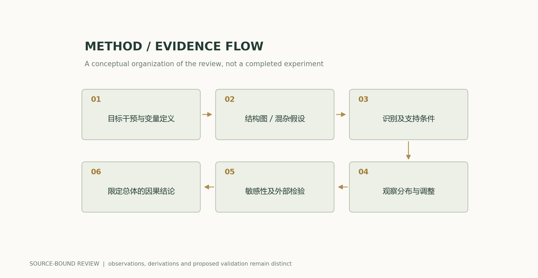
Analytical figures and numerical examples
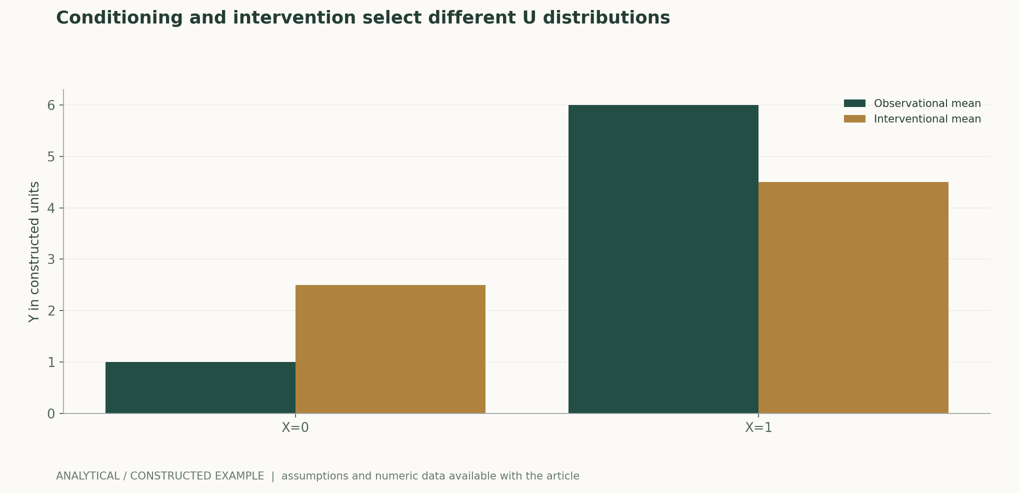
Recalculable worked example
The observational means are 1 and 6, a difference of 5; the interventional means are 2.5 and 4.5, a difference of 2. Backdoor weighting recovers the interventional means using the population distribution of U, but whether adjustment is possible in reality still requires causal assumptions.
Comparison of methods
| Method or judgment | Control variables and measurement | Failure conditions and interpretation |
|---|---|---|
| Observational prediction | Report P(Y|X) and the data source | Predictive accuracy does not identify intervention effects |
| Backdoor adjustment | Provide the graph, adjustment set, and support conditions | Incorrect control can increase bias |
| Latent representations | List identification assumptions and equivalent solutions | An interpretable name does not make a causal variable |
| Cross-domain stability | Design environments and controlled comparisons of competing explanations | Stable accuracy alone does not establish causality |
Verification and experimental plan
- Define the target population, treatment, outcome, timing, and effect to be estimated.
- Diagram the causal assumptions and temporal ordering of variables, and document risks of hidden confounding.
- Check the adjustment set, consistency, positive support, measurement error, and missingness mechanism.
- First check the estimator using exhaustively enumerable simulations, then analyze lawful data.
- Conduct sensitivity analyses, negative-control tests, or external intervention tests, retaining competing explanations.
- When identification is not possible, explicitly report associations or bounds, rather than rewriting predictions as causal conclusions.
Scope and limitations
- The model and probabilities are entirely constructed.
- No real intervention effects have been estimated.
- Identification assumptions generally cannot be proven by data alone.
- Cross-domain prediction does not automatically establish causal structure.
Mapping primary sources to claims
- Towards Causal Representation LearningBernhard Schölkopf, Francesco Locatello, Stefan Bauer, Nan Rosemary Ke, Nal Kalchbrenner, Anirudh Goyal, Yoshua Bengio · 2021-02-22Abstract and sections on interventions, independent mechanisms and causal representations
- Invariant Risk Minimization, , , · 2019-07-05Abstract; 原文方法、理论和实验章节见作者原始论文链接
- WILDS: A Benchmark of in-the-Wild Distribution Shifts, , , , , , , , , , , , , , , , , , , , , , -------------------------------------------------------------------------------- · 2020-12-14Abstract; 原文方法、理论和实验章节见作者原始论文链接
Citation and manuscript export
BibTeXRISCSL JSONTXTArticle JSON
Author, version, and sources
An AI-assisted research review; Codex (AI) wrote the article and performed analytical derivations based on the listed primary literature. This site has no record of independent peer review or original model experiments for this article.
Reader performance revision: previously read pages are also reused when a recent HEAD request returns 200 and the ETag matches. The main text, equations, sources, and scientific figure data retain the content of the previous version.
The conceptual cover is separate from the scientific diagrams; scientific figures are calculated from disclosed equations and explicit assumptions, and all results from original papers are attributed to their sources.
Author, version, and correction history · /guides/causal-inference-ai/v1/
Sources for the cover and scientific figures · Data, sources, and assumptions · Publication and version history
Source revision: 6251a250b27bb8b449f59b392f81abd355383770