

Abstract
Neural scaling laws turn resource allocation into a quantitative problem, but an optimum is only as meaningful as its objective and accounting boundary. We derive the allocation implied by a separable power-law loss under a product compute constraint, then show how changing exponents, a finite data ceiling, or an inference charge changes the decision. The curves use declared dimensionless coefficients and are not fits to published model runs. Three primary sources provide empirical and theoretical context. Our contribution is a transparent sensitivity analysis and a reproducible decision procedure that separates a scaling relation, an optimization solution, and a deployment recommendation.
1. An optimum needs a complete question
The phrase compute-optimal model leaves at least three choices unstated: what quality is optimized, which resources count, and what alternatives are feasible. Minimizing held-out cross-entropy at fixed training arithmetic is different from minimizing total expenditure at a required task quality. A model that is attractive for one training run may be unattractive when queried many times.
The appropriate output of a scaling analysis is therefore a conditional decision, not a universal parameter-to-token ratio. This perspective studies a deliberately simple loss model in normalized units. It is useful because the optimum can be derived and independently checked. Its simplicity also makes omissions visible: data quality, repeated examples, context length, optimization inefficiency, and hardware utilization are not hidden inside an unexplained empirical coefficient.
2. The selected research gives context, not a universal constant
Kaplan and colleagues measured language-model loss scaling with model size, data and training compute. Hoffmann and colleagues investigated compute allocation and obtained a different practical balance between parameters and training tokens in their study. Bahri and colleagues analyzed mechanisms and regimes that can produce neural scaling behavior.
These contributions do not imply that all tasks share a single exponent or that a fitted law transfers unchanged across data pipelines and model families. We use them to motivate explicit allocation analysis, not to declare a current best model size. The numerical examples below choose their own coefficients and exponents. No displayed point is a published experimental observation, and none is a forecast for a named production model. [1], [2], [3]
3. A separable loss model exposes the tradeoff
Assume excess loss above an irreducible floor is a N to the power minus alpha plus b D to the power minus beta. Here N and D are dimensionless parameter and token counts relative to specified reference units, and all four constants are positive. Increasing either resource reduces its corresponding term, but at a fixed product budget it reduces the other resource.
The separability assumption is substantial. It excludes interactions in which additional data changes the model-size exponent, and it treats all counted tokens as equally useful. It also presumes that the selected training procedure reaches the modeled loss for each allocation. These assumptions are not consequences of a smooth plotted curve. They are hypotheses that a real fitting study would need to test using residual structure and held-out resource scales.
4. Deriving the conditional allocation
Let normalized training compute be C=kND with k>0. Eliminating D leaves aN to the power minus alpha plus b(kN/C) to the power beta. Differentiate with respect to log N. At an interior optimum, alpha times the model-limited loss contribution equals beta times the data-limited contribution.
Solving gives N proportional to C raised to beta/(alpha+beta), while D is proportional to C raised to alpha/(alpha+beta). Equal resource exponents arise when alpha and beta are equal; they are not an identity imposed by the compute constraint. The optimal ratio also depends on a, b, k and the resource units. Quoting a numeric ratio without those definitions makes it impossible to reproduce the allocation, even if the derivative calculation itself is correct.
5. A symmetric example that can be checked by hand
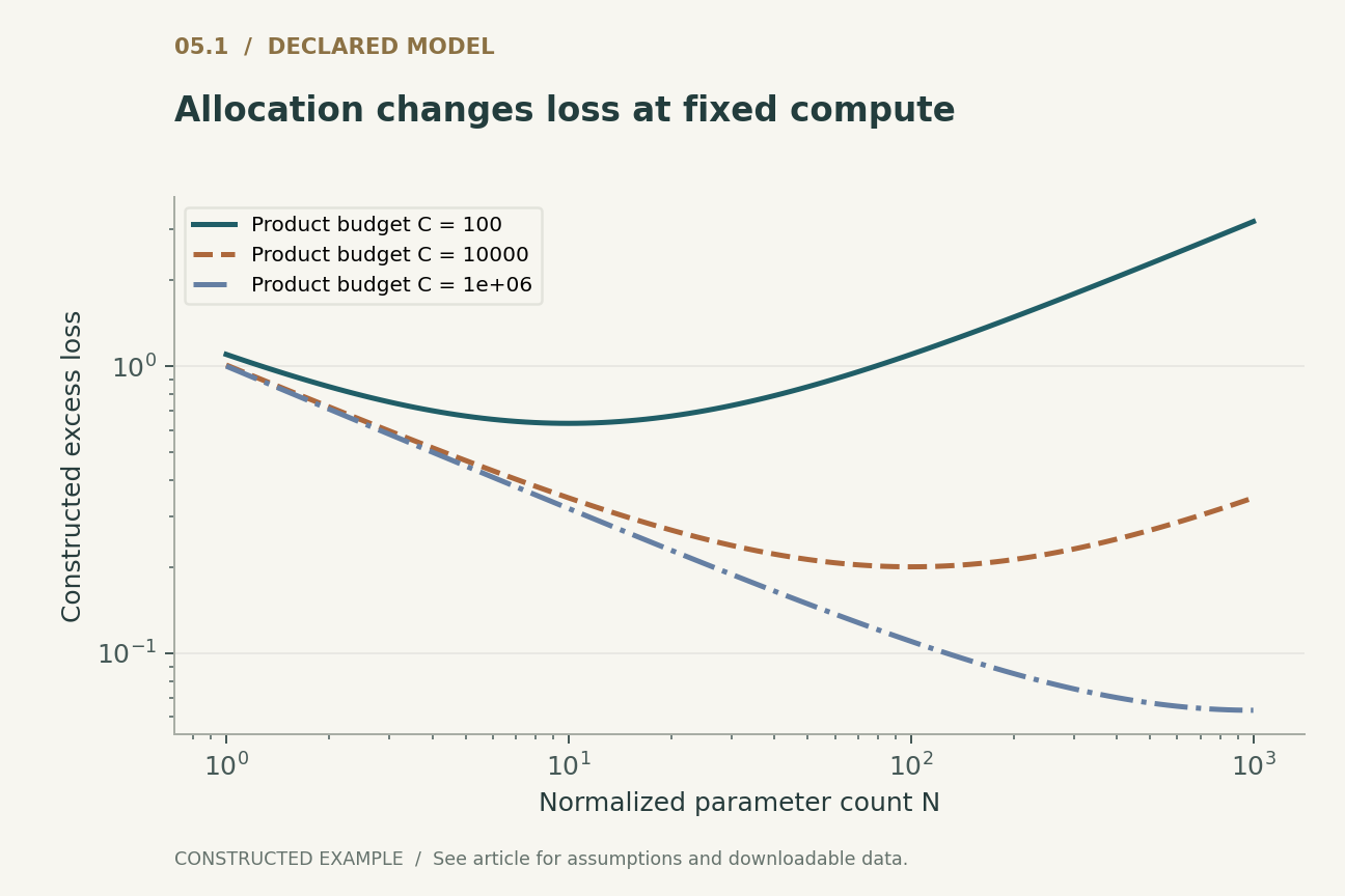
Set a=b=k=1 and alpha=beta=1/2. For C=10,000, the optimum is N=D=100 and excess loss is 0.2. This follows both from differentiation and from convexity in log N. At N=25, D=400, the excess loss is 0.25; the same value occurs at the reversed allocation.
These are normalized quantities, not billions of parameters or tokens. Their role is to show how an allocation can waste a fixed product budget. Our first plot compares several compute budgets, and the executable check compares the analytic optimum with a dense logarithmic search. The search is a numerical consistency check for this model, not an independent empirical validation of the assumed power law.
6. Exponent uncertainty becomes allocation uncertainty
Taking logarithms reveals that the predicted optimal log parameter count depends on both fitted coefficients and exponents. At large budgets, even a small uncertainty in the compute exponent can produce a substantial multiplicative change in the recommended size. A fit that looks close over observed losses can therefore imply a poorly determined extrapolated allocation.
For illustration, compare two hypothetical exponent pairs rather than fitting them to invented observations. Changing alpha while fixing beta changes the slope of log N against log C, not merely its intercept. A real analysis should propagate joint parameter uncertainty, because coefficients and exponents can be strongly correlated. Reporting only the standard error of the final loss prediction can conceal uncertainty in the decision that produced it.
7. A finite data ceiling changes the feasible set
If only Dmax distinct usable tokens are available and repetition is excluded by the model, the unconstrained optimum may demand too much data. On the boundary D=Dmax, a fixed product budget implies N=C/(kDmax). The allocation no longer follows the unconstrained interior power law. It is determined by a feasibility constraint.
Allowing repeated epochs does not automatically remove that constraint. A law fitted to distinct data cannot silently interpret repeated tokens as equally informative new examples. One would need a model of effective data or a separate experimental relation for repetition. The important point is mathematical: an optimizer must know the feasible set. Increasing a headline compute budget cannot create new independent information by itself, and a constrained solution should be labeled as such.
8. Inference costs shift the optimum
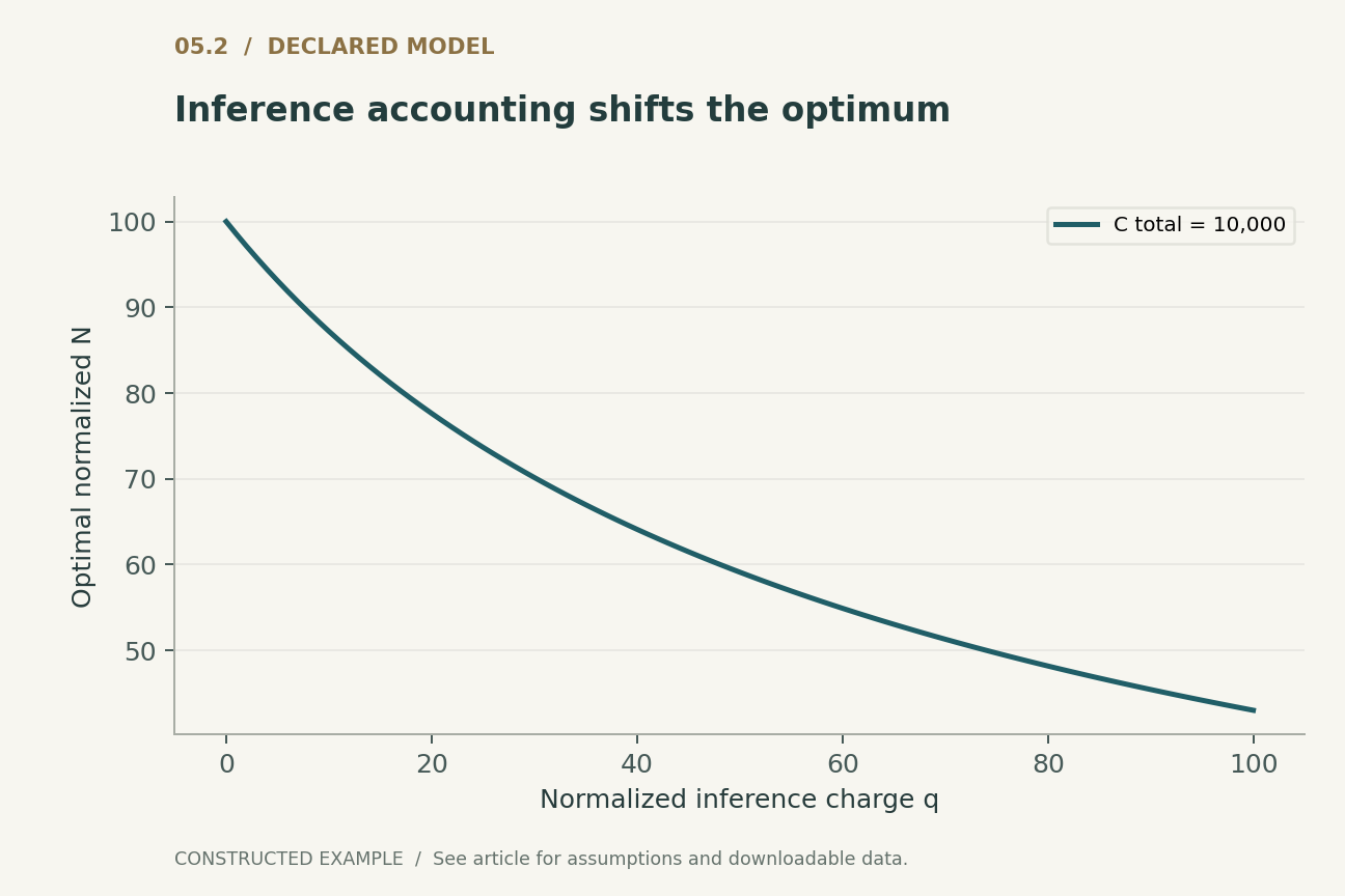
Add a normalized inference charge qN to the budget, with q representing an assumed lifetime workload and per-parameter inference coefficient. Then Ctotal=N(kD+q), so feasible data becomes (Ctotal/N-q)/k. Increasing N consumes both training product budget and an additional charge. A training-only optimum generally ceases to be optimal under this objective.
For the symmetric example at Ctotal=10,000, a positive q shifts the optimum toward a smaller N than the N=D=100 allocation obtained at q=0. The companion code solves the declared stationary equation and compares nearby feasible allocations. These are model calculations, not measured serving costs. Attention, context length, batching, memory traffic and heterogeneous requests are omitted. The example shows why the accounting boundary matters; it does not supply a production cost estimate.
9. Quality metrics cannot be interchanged for free
Cross-entropy measures an expected logarithmic score under an evaluation distribution and tokenization. An operational task may instead care about exact correctness, calibration, latency, or performance on a rare subgroup. A smooth improvement in average loss does not identify the change in each of those outcomes.
A deployment decision should either optimize the actual downstream metric or validate the mapping from the modeled loss to that metric. The validation must use data outside the fitting process. If a benchmark is selected because it favors the proposed allocation, the apparent agreement is subject to selection bias. Multiple metrics may define a Pareto frontier rather than a single optimum; the decision rule should then state whose preferences resolve the tradeoff instead of treating one scalar loss as self-evidently sufficient.
10. Testing a scaling claim requires held-out scales
A useful fitting study spans resource combinations rather than only a diagonal sequence where N and D grow together. Otherwise separate effects can be poorly identified. It should record failed runs, training schedules, effective tokens and quality filters, and should reserve resource scales or allocations for validation.
Residual plots should test systematic departures such as saturation, interaction terms, or changing exponents. Extrapolation should be bounded by the observed regime and accompanied by sensitivity to alternative models. More compute points do not automatically repair a confounded design. A small, well-chosen grid that separates model and data effects can be more informative than many runs along one resource ratio. The proposed protocol follows from this identification problem rather than from an assumption that every curve must be a power law.
11. What can be decided from the present evidence
The companion checks verify the interior solution, positive second derivative in log size, equality of weighted marginal contributions, and boundary behavior under a data cap. They also solve the inference-inclusive example independently and compare the result with nearby feasible allocations. The two figures show the declared training-only tradeoff and the changed optimum as the inference charge grows.
No large model was trained and no scaling coefficients were estimated from new observations. The conclusion is a decision discipline: first identify the quantity being optimized, then fit and challenge the response model, then solve within the actual constraints, and finally test the chosen allocation. A scaling law is valuable precisely when this chain is explicit. Without it, compute-optimal can become a label attached to an unexamined resource preference.
12. A budget inequality need not be fully spent
The positive power-law model makes additional training resources always beneficial, so an unconstrained optimum uses the available budget. Real decisions may include a quality threshold or a penalty for elapsed time, in which case leaving budget unused can be optimal. An equality constraint is consequently a modeling choice, not an obligation to spend. Before optimizing an allocation, distinguish a maximum permitted cost from a required resource expenditure.
Executed locally · Bounded scope
Allocation derivatives, data cap, and inference budget
Nine power-law coefficient/budget cases and 101 inference charges with exact stationary conditions. Does not validate the loss or cost model empirically.
342 assertions passed. These checks validate the supplied example, not the cited systems.
Inspect the recorded witness
{
  "symmetric_optimum": [
    100.0,
    100.0
  ],
  "data_cap_optimum": [
    400.0,
    25
  ],
  "inference_q100_optimum": [
    43.01597090019469,
    132.47179572447453
  ]
}
Example runner · Model loader · Training models · Representation models · Generation models · Reliability modelsRead the complete check results
A declared analytical model
Four equations, explicit assumptions
(1) Declared separable model; N,D,C normalized to fixed reference units, with positive coefficients and exponents.
(2) Interior first-order condition under the product compute constraint.
(3) Conditional training-only optimum, valid when no feasibility bound is active.
(4) Illustrative lifetime inference charge qN; q is a declared normalized constant, not a measured serving cost.
Constructed examples · Reproducible data
Inspect the quantitative argument
These curves are calculated from the declared models. They are not observations from the cited studies. Every figure includes its numeric data and vector version.


Which evidence answers which question?
| Decision model | Included costs | Missing evidence |
|---|---|---|
| Training-only product budget | kND | Deployment workload and hardware utilization |
| Data-capped allocation | Product budget and usable-data limit | Value of repeated examples |
| Lifetime simplified budget | Training plus qN inference charge | Real request mix and serving measurements |
A proposed validation protocol
This is a proposed evaluation design. No production-system or hardware benchmark was performed. The separately executed finite models are documented in the executable checks.
- Define quality, resource units, accounting boundary and feasible data supply.
- Choose a grid that varies model and data size separately.
- Record all training schedules, failed runs and effective token counts.
- Fit competing response models and inspect structured residuals.
- Propagate joint fit uncertainty into allocation uncertainty at held-out scales.
- Validate the selected allocation against actual downstream quality and measured total cost.
What the primary sources establish
Jared Kaplan, Sam McCandlish, Tom Henighan et al. · 2020 [1]
Contribution. Reports empirical power-law relationships for neural language-model losses and compute allocation.
Boundary. The fitted regime and training procedure constrain extrapolation.
Source locator. Author manuscript abstract and scaling-law formulation.
Jordan Hoffmann, Sebastian Borgeaud, Arthur Mensch et al. · 2022 [2]
Contribution. Studies allocation of parameters and tokens under training compute budgets.
Boundary. Its practical allocation is evidence for the studied setting, not a universal ratio.
Source locator. Author manuscript Section 3, especially the parametric loss formulation.
Yasaman Bahri, Ethan Dyer, Jared Kaplan et al. · 2024 [3]
Contribution. Develops explanations for multiple neural scaling regimes.
Boundary. Different mechanisms and regimes can produce different exponents.
Source locator. Author manuscript abstract and scaling-regime taxonomy; final PNAS metadata retained.
Limits of this analysis
- All numerical coefficients are illustrative and dimensionless.
- No training run or empirical scaling-law fit was performed.
- The separable loss excludes data quality, repetition and interaction effects.
- The inference charge is a simplified model, not a serving benchmark.
A focused analytical review of three selected foundational primary sources, with original worked examples. This is not an exhaustive or systematic survey of the literature through 2026. Source access and version notes are recorded with the bibliography.
Questions that would change the conclusion
- Which allocation decisions remain stable under plausible alternative loss models?
- How should data quality and repetition enter an identifiable resource model?
- When does lifetime inference dominate the economically optimal model size?
References
- Jared Kaplan, Sam McCandlish, Tom Henighan et al.. Scaling Laws for Neural Language Models. arXiv:2001.08361 (2020). 10.48550/arXiv.2001.08361.
- Jordan Hoffmann, Sebastian Borgeaud, Arthur Mensch et al.. Training Compute-Optimal Large Language Models. arXiv:2203.15556 (2022). 10.48550/arXiv.2203.15556.
- Yasaman Bahri, Ethan Dyer, Jared Kaplan et al.. Explaining Neural Scaling Laws. Proceedings of the National Academy of Sciences 121(27), e2311878121 (2024). 10.1073/pnas.2311878121.
Source [1] access. Primary bibliographic record and abstract inspected; no exhaustive full-text or supplementary-material audit.
Source [2] access. Primary record and author HTML manuscript introduction and Section 3 structure inspected. No published coefficient is used in the article figures.
Source [3] access. Primary bibliographic record and abstract inspected; no exhaustive full-text or supplementary-material audit.
Version note. Primary author record v2 (29 April 2024) supplies the final PNAS 2024 bibliographic reference; author manuscript first posted 2021.
Bibliographic identities were checked against primary publisher and author records. Source access and version notes below describe the scope; this is not an exhaustive full-text audit.
Authorship and provenance
Written and technically self-reviewed by Codex (AI). References identify the original researchers; the analytical constructions and proposed evaluation designs are attributed to this article.
Covers are conceptual ImageGen illustrations. Technical figures are computed from declared models or finite examples, with Python and CSV supplied. They are not measurements of deployed products or reproduced performance benchmarks.
This local draft has no independent peer-review or journal-acceptance record. Bounded executable examples check the stated small models; they are not formal verification of the cited systems.