

Abstract
Diffusion models decompose a complex generation problem into multiple denoising problems under noisy conditions, but training loss, sampling paths, and final visual quality are not the same quantity. Starting from the closed-form marginal distribution of the Gaussian forward process, this article analyzes the relationship between noise parameterization and the signal-to-noise ratio, then discusses how few-step sampling, conditional guidance, and latent-space compression introduce different approximations. The analytical figures disclose the noise schedule, number of steps, and calculation method to illustrate mechanisms; this article trains no diffusion network and makes no claim to new image-generation quality results.[1] Denoising Diffusion Probabilistic Models[2] Score-Based Generative Modeling through Stochastic Diff[3] High-Resolution Image Synthesis with Latent Diffusion M
English abstract
Diffusion models are examined as learned denoising processes with an explicitly chosen noise schedule. We separate training objectives, discretization, guidance and latent compression. Analytical signal-to-noise curves use a declared schedule and contain no generated-image benchmark results. The proposed evaluation controls the decoder, sampling budget and conditioning before attributing differences to a sampler.
1. The Forward Process First Defines the Learning Problem
In classical discrete diffusion, the forward process progressively adds Gaussian noise according to preset variances. Multiple Gaussian transformations can be combined into a closed-form distribution conditioned on the original image, so training need not actually execute all perturbation steps consecutively. The noise schedule defines how much original information can be retained at different time points and determines the difficulty encountered by training samples. The same time index does not imply the same noise level across different schedules; model comparisons should retain the cumulative signal coefficient or log signal-to-noise ratio, rather than merely specifying a step number. The forward schedule is manually specified; it is the reverse process that is learned from data.[1] Denoising Diffusion Probabilistic Models
2. Noise Prediction and Image Error Have Different Weights
If the network predicts noise, an estimate of the original image can be recovered from the noisy input and predicted noise. Substitution into the closed-form distribution shows that the original-image estimation error equals the noise-prediction error multiplied by a time-dependent coefficient. Thus, a simple average of noise mean squared error is not equivalent to original-image mean squared error with equal weights across all time points. The training objective may also derive from a weighted form of a variational bound. When reading papers, one should distinguish the derived objective, the simplified loss actually used, and the time-point sampling distribution; reporting a decrease in a training loss alone cannot establish comprehensive improvements in visual detail or conditioning fidelity.[1] Denoising Diffusion Probabilistic Models
3. The Learned Denoiser Does Not Uniquely Determine the Sampling Trajectory
DDIM shows that, in a construction compatible with the training marginal distributions, sampling paths different from the original Markov reverse chain can be used, with deterministic updates obtainable under particular settings. Reducing the number of steps changes the discrete approximation, and errors depend not only on the network but also on the arrangement of time points, the update rule, and randomness. Fixing a random seed only constrains random inputs within the same implementation; it does not automatically make different samplers equivalent experiments. A fair comparison should hold conditioning, the network, the decoder, and the budget fixed, and report the actual number of network evaluations and total elapsed time, rather than listing only a nominal step count.[2] Score-Based Generative Modeling through Stochastic Diff[1] Denoising Diffusion Probabilistic Models
4. Guidance and Compression Require Separate Explanations
Conditional guidance often changes the direction of generation by combining predictions under different conditions; stronger guidance may improve condition matching while changing diversity or causing problems such as saturation. Latent diffusion first uses an encoder to map images to lower-dimensional representations and then learns diffusion in latent space; its computational savings arise from joint changes in the representation and network. Compression may lose small text, fine geometry, or rare structures. If the decoder already cannot faithfully reconstruct a class of inputs, output defects cannot all be attributed to denoising sampling, nor can image-space quality be compared on the basis of latent-space loss alone.[3] High-Resolution Image Synthesis with Latent Diffusion M
5. Quality Metrics Must Match the Questions of Use
Distribution-distance metrics, per-sample similarity, text matching, and human preference address different questions. Preprocessing and the evaluation encoder should be frozen, sample sizes and randomized repetitions disclosed, and filtering and manual image-selection rules stated before the results. Showing only a few selected images conceals failure cases in the generation distribution. Tasks involving text, counting, or spatial relations require dedicated, verifiable tests; nearest neighbors in the training data and data provenance should also be examined to distinguish generative capability from memorized reproduction. This article's signal-to-noise curves analyze a schedule and cannot replace any of these image-quality evaluations.[1] Denoising Diffusion Probabilistic Models[3] High-Resolution Image Synthesis with Latent Diffusion M
6. Boundaries Between Mechanistic and Empirical Conclusions
The forward equations allow the signal-to-noise ratio of a schedule to be calculated exactly and the algebraic relationship between noise error and original-image error to be proved; these results do not imply that a particular sampler must perform better on real-world images. Network approximation error varies with the data, parameterization, and training resources, and the decoder introduces additional error. A complete study should first check the implementation against the equations, then test empirical hypotheses using a fixed model and independent samples. Equation verification, numerical-stability verification, and generation-quality verification should be documented separately, so that success in one form of verification is not repurposed as a conclusion of another kind.[1] Denoising Diffusion Probabilistic Models[2] Score-Based Generative Modeling through Stochastic Diff[3] High-Resolution Image Synthesis with Latent Diffusion M
Core Equations and Derivations
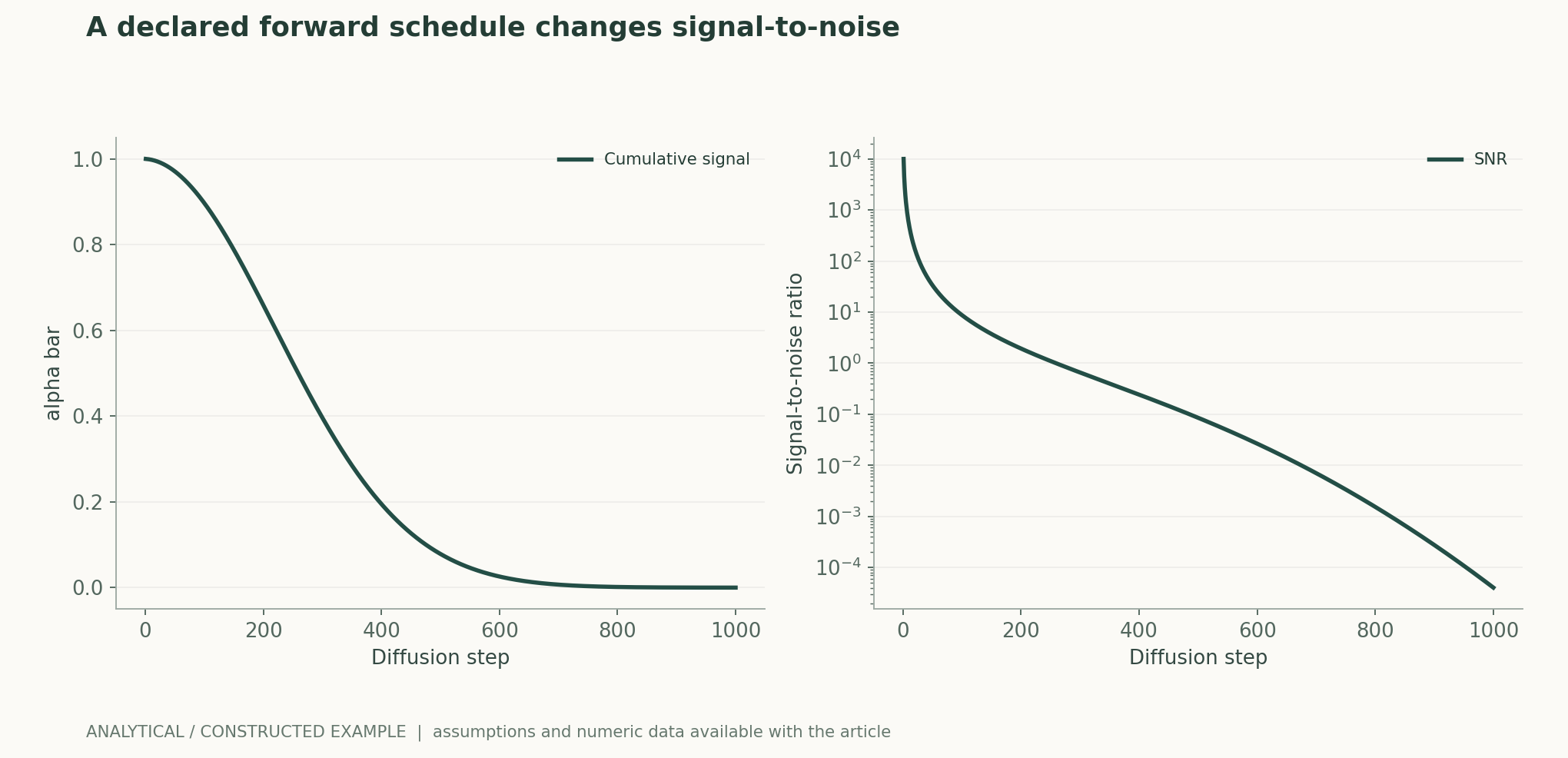
(1) Closed-form marginal distribution of linear Gaussian perturbation; the figure uses 1000 steps, with β increasing linearly from 0.0001 to 0.02. This is a chosen schedule, not a conclusion of optimality.
LaTeX
q(x_t\mid x_0)=\mathcal N(\sqrt{\bar\alpha_t}x_0,(1-\bar\alpha_t)I),\quad\bar\alpha_t=\prod_{s=1}^{t}(1-\beta_s)(2) Holds for the same noisy sample and true noise, revealing time-dependent loss weights; noise MSE cannot be directly treated as equally weighted original-image error across time points.
LaTeX
\hat x_0=\frac{x_t-\sqrt{1-\bar\alpha_t}\,\epsilon_\theta(x_t,t)}{\sqrt{\bar\alpha_t}},\quad\|\hat x_0-x_0\|^2=\frac{1-\bar\alpha_t}{\bar\alpha_t}\|\epsilon_\theta-\epsilon\|^2(3) Assumes unit variance of the original signal and represents the theoretical ratio in the forward process, not image-reconstruction quality or human preference.
LaTeX
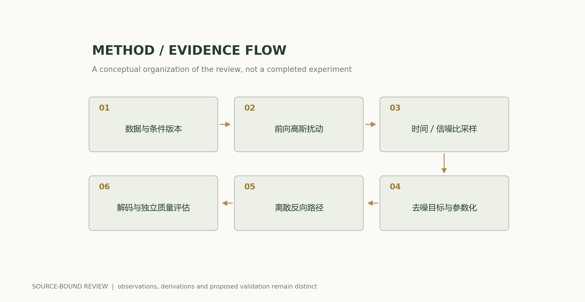
\operatorname{SNR}_t=\bar\alpha_t/(1-\bar\alpha_t)Method and Evidence Workflow
Analytical Figures and Numerical Examples
Recalculable Worked Example
Under the declared schedule, the cumulative signal coefficient at step 500 is 0.07859, and the SNR is approximately 0.08529. These values are determined solely by β and do not include denoising error, the decoder, or image quality.
Method Comparison
| Method or Judgment | Controlled Variables and Measurements | Failure Conditions and Interpretation |
|---|---|---|
| Noise schedule | Retain β or log SNR and the time-sampling distribution | The same number of steps does not guarantee the same noise-related difficulty |
| Few-step sampling | Fix the network, conditioning, and number of evaluations | Speed changes cannot be explained by nominal step counts alone |
| Latent-space generation | Measure encoder/decoder reconstruction error separately | Compression loss and diffusion error can become mixed |
| Quality evaluation | Report distribution, diversity, and conditioning fidelity separately | Selected examples do not represent the generation distribution |
Verification and Experimental Plan
- Freeze the versions of the model, encoder, decoder, conditioning, and preprocessing, and retain a hash for each.
- Disclose β, cumulative α, sampling time points, and network parameterization; check the marginal distributions first.
- Compare samplers using the same batch of conditions and random inputs fixed in advance, with no selection after viewing the results.
- Record the actual number of network evaluations, device, batch size, numerical precision, and end-to-end elapsed time.
- Evaluate reconstruction, condition adherence, diversity, failure rate, and training-data nearest neighbors separately, retaining the indices of all samples.
- Repeat with independent seeds and report uncertainty, explicitly stating that this article's analytical figures cannot support quality rankings.
Scope and Limitations
- No network training or empirical measurement of generation quality was performed.
- The illustrated schedule is merely a declared choice.
- Analytical SNR does not predict semantic fidelity.
- Compression, guidance, and sampling errors require separate examination.
Primary Sources and Corresponding Claims
- Denoising Diffusion Probabilistic Models, , · 2020-06-19Abstract; 原文方法、理论和实验章节见作者原始论文链接
- Score-Based Generative Modeling through Stochastic Differential Equations, , , , , · 2020-11-26Abstract; 原文方法、理论和实验章节见作者原始论文链接
- High-Resolution Image Synthesis with Latent Diffusion Models, , , , · 2021-12-20Abstract; 原文方法、理论和实验章节见作者原始论文链接
Citation and Manuscript Export
BibTeXRISCSL JSONTXTArticle JSON
Author, Version, and Sources
AI-assisted research review; Codex (AI) wrote the article and performed analytical derivations based on the listed primary literature. This site has no record of independent peer review or original model experiments for this article.
Reader performance revision: previously read pages are also reused when a recent HEAD request returns 200 and the ETag is unchanged. The main text, equations, sources, and scientific-figure data retain the content of the previous version.
The conceptual cover is separate from the scientific diagrams; scientific figures are calculated from disclosed equations and explicit assumptions, and results from original papers are attributed to their sources.
Author, Version, and Correction History · /guides/diffusion-foundations/v1/
Cover and Scientific-Figure Sources · Data, Sources, and Assumptions · Publication and Version History
Source revision: 6251a250b27bb8b449f59b392f81abd355383770