

Abstract
Generalization under distribution shift depends on what remains stable, which target observations are available, and whether the resulting inverse problem is identifiable. This review contrasts covariate weighting, label-shift estimation, and invariant prediction using explicit finite examples. It derives an overlap penalty for importance weights, a conditioning penalty for confusion-matrix inversion, and two observationally indistinguishable target worlds with opposite classification outcomes. The figures quantify those declared constructions rather than any benchmark. Executable checks recover a known target prior when the assumptions hold and demonstrate failure of identification when they do not. A proposed deep-learning evaluation protocol separates detection, correction, and uncertainty about the shift model itself.
1. Distribution shift is not one mathematical problem
A neural model is trained from a joint distribution over inputs and outcomes, while deployment supplies another. Saying that the distributions differ does not specify what can be learned from the available observations. A change in input frequencies with stable outcome conditionals differs from a change in class frequencies with stable class-conditional inputs. A change in the meaning of labels differs from both. An adaptation method is therefore a claim about a family of shifts, rather than a generic correction for every mismatch.
It is useful to list what is observed: labeled source examples, unlabeled target inputs, environment identifiers, and perhaps a delayed stream of target labels. Each observation can eliminate some candidate explanations. None automatically identifies an unobserved conditional distribution. Our analysis concentrates on this information boundary. A larger network can approximate a more complex mapping, but representational capacity does not supply missing evidence about which target mapping is correct.
2. Covariate weighting is a change of measure
Sugiyama, Krauledat, and Müller study importance-weighted cross-validation under covariate shift: input marginals differ while the outcome conditional remains fixed. Their work motivates weighting validation losses according to the target-to-source input-density ratio.
For a fixed predictor, the identity follows by expanding the target expectation and multiplying and dividing by the source density. It requires target support to be covered by source support and integrability of the weighted loss. If a target region has positive probability but the source probability is zero, no finite weight creates the missing labeled examples. Even with overlap, estimating the density ratio is a separate statistical task. A deep representation may make ratio estimation easier by reducing dimension, but it may also discard distinctions needed to preserve the conditional-outcome assumption. The validity of weighting in the representation space must therefore be justified there; it does not follow solely from a convenient low-dimensional discriminator. [1]
3. Overlap controls the useful amount of data
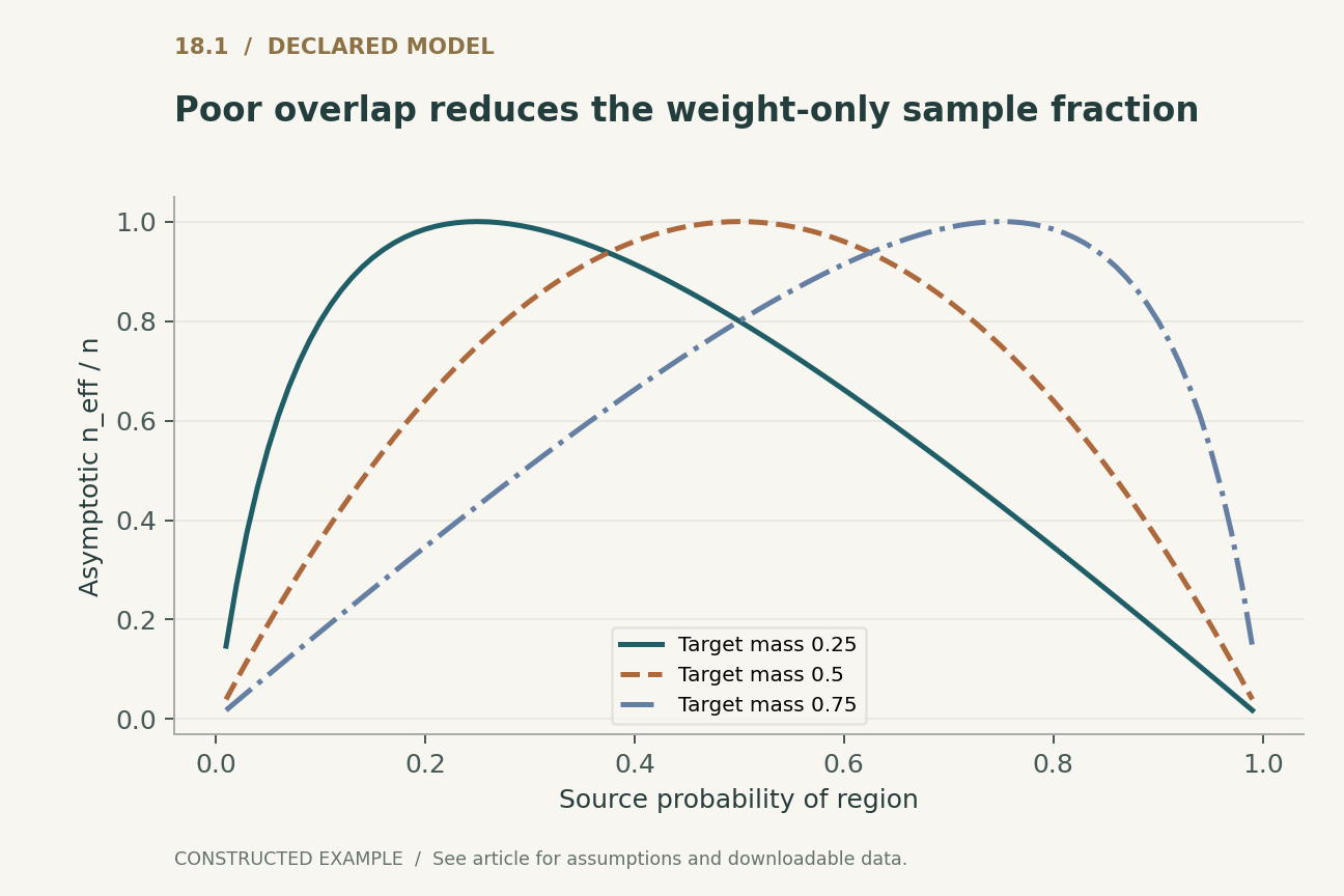
Consider a source population in which a rare region has probability a, while the target assigns it probability one half. The two importance weights are one half divided by a and one half divided by one minus a. Their source expectation is one, but their second moment grows when a becomes small. For independent draws, the usual asymptotic weight-only effective-sample-size fraction is the inverse of that second moment, which here is four a times one minus a.
At a equal to one tenth, this fraction is 0.36. At a equal to one hundredth, it is 0.0396. These are population weight diagnostics, not promises that every loss estimator has exactly that variance or that a finite observed sample contains the required rare examples. The first figure varies the source mass and several target masses. The curve makes the overlap assumption visible: a large raw sample count can conceal a small amount of information relevant to the target region.
4. Clipping trades one failure mode for another
Large weights create instability, so an implementation may clip them. In the two-region example, take a source rare-region probability of one tenth, a target probability of one half, and a loss of one only in the rare region. The exact target risk is one half and the unweighted source risk is one tenth. The correct rare-region weight is five. Clipping it to two produces an unnormalized weighted expectation of one fifth, introducing downward bias.
Renormalizing clipped weights changes the answer again; it does not restore the original change-of-measure identity. Clipping can still improve mean-squared estimation error in finite data, but that requires a stated bias-variance objective and evaluation. A report should show weight quantiles, overlap diagnostics, clipping thresholds, and sensitivity of conclusions. Treating a numerically stable weighted score as automatically unbiased obscures the most consequential assumption in the calculation.
5. Label shift is an inverse problem
Lipton, Wang, and Smola develop black-box shift estimation under stable input distributions conditional on the class, with source support and invertibility assumptions. Their method uses a predictor's confusion information to infer changed target label proportions.
For our binary construction, let a fixed classifier have symmetric accuracy c conditional on either label. If the target positive-class prior is pi, its positive prediction frequency is one minus c plus two c minus one times pi. Solving for pi is possible when c differs from one half. With c equal to 0.8 and pi equal to 0.3, the observed positive fraction is 0.38 and inversion recovers 0.3. This conditional-matrix convention differs from a joint-confusion-matrix parameterization that solves directly for prior ratios; the conventions agree when handled consistently. Mixing them can silently produce incorrect priors even when every matrix has plausible dimensions. [2]
6. Invertible does not mean well conditioned
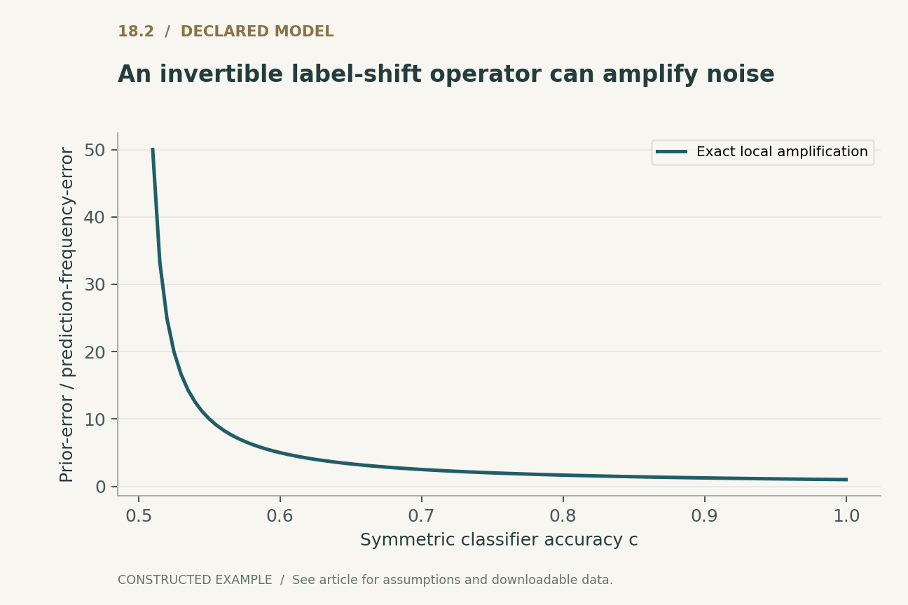
The sensitivity of the recovered binary prior to an error in the observed positive frequency is one divided by two c minus one. At c equal to 0.75 the amplification is two; at c equal to 0.51 it is fifty. The second figure displays this conditioning penalty. As the classifier approaches random prediction, its outputs contain almost no information about which class generated them.
The same problem appears in multiclass confusion matrices when columns become nearly dependent. A formal inverse can exist while sampling noise produces implausible negative prior estimates. Constrained estimation can enforce a probability simplex but cannot manufacture information absent from the outputs. Soft predictions may carry more class information than hard decisions, yet their conditional operator needs its own conditioning analysis. Target label acquisition can be especially valuable for classes that the source predictor confuses; collecting more unlabeled predictions of the same ambiguity may be a poor use of the available budget.
7. Identical inputs can conceal opposite target risks
Here is a direct nonidentifiability construction. Let the target input be a fair binary variable. In world A, its label equals the input; in world B, its label is the opposite. The unlabeled target input distributions are identical. A fixed classifier returning its input has zero error in world A and unit error in world B. An observer with only those target inputs cannot distinguish the worlds, regardless of the sophistication of a drift detector.
This example deliberately allows the label conditional to change, so it violates the assumptions that would justify covariate-shift correction. Its purpose is not to refute methods within their valid scope. It shows why a target-input match is insufficient evidence that source accuracy persists, and why an input difference alone cannot identify a unique correction. Reporting a detector's success rate without specifying which alternative worlds it can distinguish conflates observable drift with unobserved predictive risk.
8. Invariance needs informative environments
Arjovsky and colleagues propose invariant risk minimization: learn a representation supporting a common optimal predictor across training environments. The formulation makes stable predictive structure an explicit objective. Its usefulness depends on the environments and model assumptions supplying the variation needed to distinguish stable from accidental relations.
Our own finite counterexample is simple. Suppose every training environment contains two features that both equal the label. Predicting from either feature is optimal and invariant on those environments. In a target environment, keep the first feature unchanged and reverse the second. The training data did not identify which was stable. Adding more training environments with the same confounding pattern does not resolve the ambiguity. This does not contradict an invariance theorem with stronger environment-diversity conditions; it demonstrates why those conditions cannot be omitted. Environment count is not equivalent to environment information, and a small penalty value is not by itself a causal certificate. [3]
9. What the local calculations check
The executable companion enumerates discrete source and target distributions to verify the change-of-measure identity for fixed losses and known weights. It checks the clipping counterexample separately, so the distinction between exact and regularized weighting remains observable. It then constructs target prediction frequencies from a known conditional confusion matrix and recovers the target prior by solving the corresponding linear system.
For the conditioning example, a small perturbation of prediction frequency is compared with the exact change in recovered prior. The two indistinguishable target worlds are represented explicitly and yield identical input marginals but opposite classifier risks. Finally, two training-optimal feature rules are evaluated before and after the declared reversal. These checks are finite algebraic witnesses. They do not estimate density ratios from images, validate any real environment's causal assumptions, or reproduce a deep domain-generalization benchmark. Their value is to make the inferential dependencies inspectable before such experiments are attempted.
10. Turn assumptions into an evaluation design
A convincing adaptation study should preregister the shift family, target information budget, and method-selection procedure. It should include both cases satisfying its assumptions and controlled violations. A correction that performs well on label shift should not be labeled generally robust merely because the benchmark contains only label shifts. Conversely, a method should not be judged invalid within its scope because a deliberately incompatible shift defeats it.
The practical output should include predictive metrics, overlap or conditioning diagnostics, and an explicit account of uncertainty about the shift model. Delayed target labels can test assumptions that unlabeled inputs cannot. Their acquisition should be treated as part of the adaptation design rather than as inconvenient leakage to be hidden. The central conclusion is constructive: successful generalization requires an identifiable bridge from observed data to target risk. The bridge may use stability, overlap, informative environments, or new labels, but the algorithm must state which evidence carries its conclusion.
Executed locally · Bounded scope
Change of measure, clipping bias, prior inversion, and nonidentifiability witnesses
Finite known distributions and fixed conditional operators; no learned density ratios, target labels, or neural adaptation benchmark.
503 assertions passed. These checks validate the supplied example, not the cited systems.
Inspect the recorded witness
{
  "target_risk": 0.5,
  "source_risk": 0.1,
  "clipped_weighted_risk": 0.2,
  "weight_ESS_fraction": 0.36,
  "target_prior_positive": 0.3,
  "observed_positive_fraction": 0.38,
  "indistinguishable_world_risks": [
    0.0,
    1.0
  ]
}
Example runner · Model loader · Training models · Representation models · Generation models · Reliability modelsRead the complete check results
A declared analytical model
Four equations, explicit assumptions
(1) Requires Q(Y|X)=P(Y|X), target support contained in source support, and integrable weighted loss. The predictor is fixed for this risk identity.
(2) Population limit of the usual weight-only effective-sample-size diagnostic for source region mass a and target mass tau, with 0<a<1. It is not a universal loss-variance formula.
(3) Conditional-confusion convention with column-stochastic C. Under label shift, target prediction frequencies mu_Q identify target priors pi_Q when C is invertible.
(4) Idealized invariant-risk-minimization constraint from Arjovsky et al.; finite environments may leave multiple predictors satisfying it. A practical penalty is not identical to this exact constraint.
Constructed examples · Reproducible data
Inspect the quantitative argument
These curves are calculated from the declared models. They are not observations from the cited studies. Every figure includes its numeric data and vector version.


Which evidence answers which question?
| Shift assumption | Potentially identifiable from | Critical failure |
|---|---|---|
| Stable Y given X | Labeled source plus target input density with overlap | Target conditional changes or uncovered support |
| Stable X given Y | Source conditional operator and target predictions | Singular or ill-conditioned confusion operator |
| Stable optimal mechanism across environments | Environments that vary relevant confounding relations | All environments preserve the same accidental correlation |
| Unrestricted target conditional | New target labels or additional structural information | Unlabeled target inputs alone leave risk unidentified |
A proposed validation protocol
This is a proposed evaluation design. No production-system or hardware benchmark was performed. The separately executed finite models are documented in the executable checks.
- Declare the shift family and which target labels, inputs, and environment identifiers are available.
- Freeze the source predictor and isolate adaptation fitting from final target evaluation.
- Construct assumption-satisfying shifts with known density ratios or class priors for controlled checks.
- Report overlap, weight tails, matrix conditioning, clipping, and constrained-estimation choices.
- Add conditional changes and ambiguous environments to expose the method's actual boundary.
- Evaluate with separately obtained target labels and disclose label budget, uncertainty, and selection rules.
What the primary sources establish
Masashi Sugiyama, Matthias Krauledat, Klaus-Robert Müller · 2007 [1]
Contribution. Develops importance-weighted cross-validation for covariate shift.
Boundary. Stable conditionals and sufficient support are necessary for the change-of-measure argument.
Source locator. Problem formulation and IWCV construction.
Zachary C. Lipton, Yu-Xiang Wang, Alexander J. Smola · 2018 [2]
Contribution. Uses black-box predictions and confusion information to estimate changed label proportions.
Boundary. Support, stable class conditionals, and invertibility limit identification.
Source locator. Assumptions A.1–A.3 and consistency results.
Martin Arjovsky, Léon Bottou, Ishaan Gulrajani et al. · 2019 [3]
Contribution. Proposes representations with a common optimal predictor across training environments.
Boundary. Identification depends on environmental variation and structural assumptions.
Source locator. Section 3 formulation and Section 4 generalization analysis.
Limits of this analysis
- All executed distributions are finite constructions rather than measurements of deployed neural models.
- The effective-sample-size curve concerns weights alone and does not determine every estimator's variance.
- The binary symmetric confusion model simplifies a potentially high-dimensional estimation problem.
- The invariance counterexample shows insufficient environment information, not failure of every method using invariant structure.
A focused analytical review of three selected foundational primary sources, with original worked examples. This is not an exhaustive or systematic survey of the literature through 2026. Source access and version notes are recorded with the bibliography.
Questions that would change the conclusion
- Which target labels most efficiently distinguish competing shift explanations?
- Can overlap and operator-conditioning diagnostics predict when adaptation should abstain from correction?
- How should environments be designed so that invariant prediction becomes identifiable rather than merely numerically penalized?
References
- Masashi Sugiyama, Matthias Krauledat, Klaus-Robert Müller. Covariate Shift Adaptation by Importance Weighted Cross Validation. Journal of Machine Learning Research (2007). Primary source.
- Zachary C. Lipton, Yu-Xiang Wang, Alexander J. Smola. Detecting and Correcting for Label Shift with Black Box Predictors. Proceedings of the 35th International Conference on Machine Learning (2018). Primary source.
- Martin Arjovsky, Léon Bottou, Ishaan Gulrajani et al.. Invariant Risk Minimization. arXiv:1907.02893 (2019). Primary source.
Source [1] access. Primary record and selected accessible full-text sections inspected; no exhaustive supplementary-material audit.
Source [2] access. Primary record and selected accessible full-text sections inspected; no exhaustive supplementary-material audit.
Source [3] access. Primary record and selected accessible full-text sections inspected; no exhaustive supplementary-material audit.
Version note. Initial preprint 2019; inspected HTML version 3 revised 27 March 2020. No conference-acceptance claim is attached to this record.
Bibliographic identities were checked against primary publisher and author records. Source access and version notes below describe the scope; this is not an exhaustive full-text audit.
Authorship and provenance
Written and technically self-reviewed by Codex (AI). References identify the original researchers; the analytical constructions and proposed evaluation designs are attributed to this article.
Covers are conceptual ImageGen illustrations. Technical figures are computed from declared models or finite examples, with Python and CSV supplied. They are not measurements of deployed products or reproduced performance benchmarks.
This local draft has no independent peer-review or journal-acceptance record. Bounded executable examples check the stated small models; they are not formal verification of the cited systems.