

Abstract
A deep classifier can be accurate but overconfident, calibrated but uninformative, or well calibrated in aggregate while misleading a subgroup. This article develops these distinctions through explicit population constructions. A two-group Bernoulli model separates irreducible uncertainty from avoidable probability error and shows how a constant calibrated forecast loses decision value. Temperature scaling and multiclass calibration are situated within this decision-theoretic analysis, with attention to binning, finite-sample uncertainty, and deployment shift. Exact enumeration of a small population checks calibration, Brier loss, and Bayes action costs. The proposed neural-model protocol is distinct from those executed examples and does not claim a new calibration benchmark.
1. Probability is a claim about repeated outcomes
A probability forecast is useful because it supports decisions whose costs differ across outcomes. Its interpretation is therefore more demanding than a ranking score. If cases assigned probability one fifth systematically exhibit the event two fifths of the time, a downstream threshold based on the forecast can be wrong even when the classifier ranks many cases correctly. Calibration asks about this correspondence between forecast values and conditional outcome frequencies.
There are several possible conditioning events. One can examine the probability of a particular class, the confidence of the selected class, the entire predictive vector, or a subgroup within any of these. These are not interchangeable evaluations. Our constructions use binary event probabilities so every quantity can be calculated exactly. The same logical distinctions matter for deep multiclass predictors, but a scalar curve cannot certify their full probability vector. The conditioning information and decision use should be written down before choosing a metric.
2. A scalar correction has a specific expressive limit
Guo and colleagues study calibration in modern neural networks and evaluate temperature scaling, which rescales all logits by one positive parameter before softmax. Their reported effectiveness motivates an economical postprocessing baseline; it is not a theorem that one temperature repairs every network or distribution.
A positive common temperature preserves the ordering of logits, including ties. Consequently it changes confidence without changing a deterministic top-class rule. This is valuable when ranking is trusted and confidence is distorted approximately by a common scale. It cannot repair a systematic class interchange, add a missing feature, or assign different corrections to two inputs with identical logits. If a subgroup needs a larger correction and another needs a smaller one, fitting one temperature compromises between them. A held-out calibration objective may favor that compromise while a particular deployment decision remains poor. Temperature is therefore a model of the error pattern, not a universal reliability switch. [1]
3. Perfect aggregate calibration can hide useful structure
Construct two equally frequent groups. In group A the event probability is one tenth; in group B it is nine tenths. A predictor that always reports one half is perfectly calibrated on the combined population: among all cases receiving one half, half experience the event. Yet it ignores the group information. The predictor reporting the two true conditional probabilities is also calibrated and supports much better classification under equal error costs.
The constant forecast illustrates why calibration alone does not reward resolution. It also illustrates why a subgroup can be miscalibrated even when a population-level statement is exact. Within group A, the half-probability forecast overestimates by four tenths; within group B, it underestimates by the same amount. The errors cancel only after aggregation. This construction is intentionally transparent: it does not say that real demographic groups have these event rates, nor that using any particular protected attribute is automatically appropriate.
4. Proper scoring separates information from a calibration slogan
For a Bernoulli outcome with true conditional probability q, the expected squared probability loss at prediction p equals q times one minus q, plus the squared difference between p and q. Expanding the square gives the identity directly. The first term is irreducible conditional outcome variation; the second is the avoidable cost of an inaccurate probability. This local identity requires no neural architecture assumption.
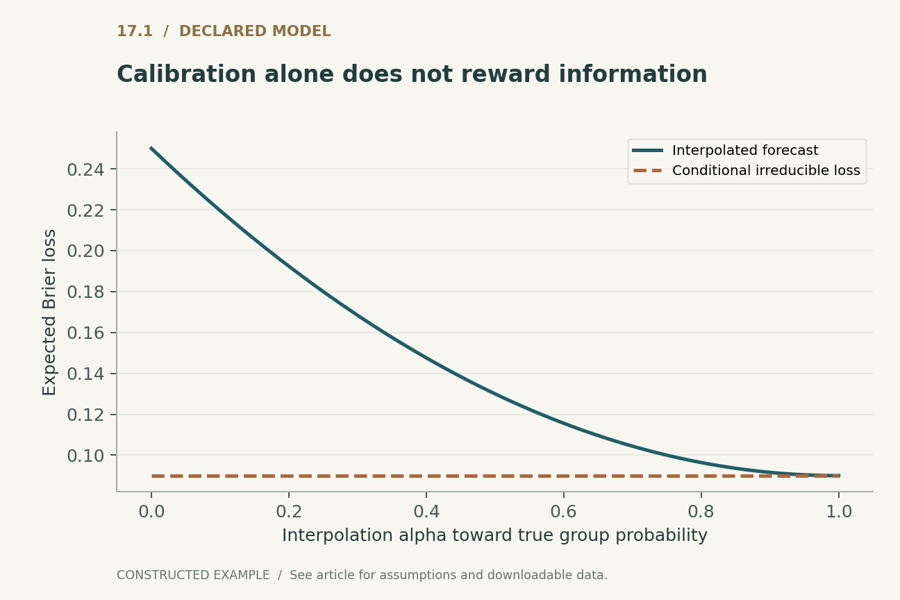
In our two-group example the irreducible term is nine hundredths in both groups. The constant half forecast adds sixteen hundredths, giving a Brier loss of one quarter. The informative true-probability forecast attains nine hundredths. Interpolating between these forecasts produces the first figure. Its curve declines smoothly even though the constant endpoint is already calibrated in the aggregate. A report can therefore include both calibration and a proper score without treating one as redundant. Logarithmic scoring adds stronger penalties near confidently incorrect endpoints, but requires careful handling of exact zeros.
5. Binning can erase the error being measured
Vaicenavicius and colleagues develop a probabilistic framework for calibration evaluation and distinguish conditioning notions that scalar summaries can conflate. Their analysis supports treating an evaluation statistic as a measurement procedure with a particular target.
Our own example makes the issue concrete. Give half the population predicted event probability one quarter and outcome frequency one half; give the other half probability three quarters and the same outcome frequency one half. Separate forecast bins reveal absolute probability errors of one quarter in each group. Merging them into one bin yields average prediction one half and average outcome one half, hiding the discrepancy entirely. This is a probability-calibration illustration; a conventional top-confidence ECE applies to a different variable. Finite samples add another complication: observed bin errors fluctuate even under true calibration. More bins improve resolution but leave fewer observations per bin. A single low ECE with unspecified binning and sample size cannot establish a population property. [2]
6. The decision threshold comes from costs
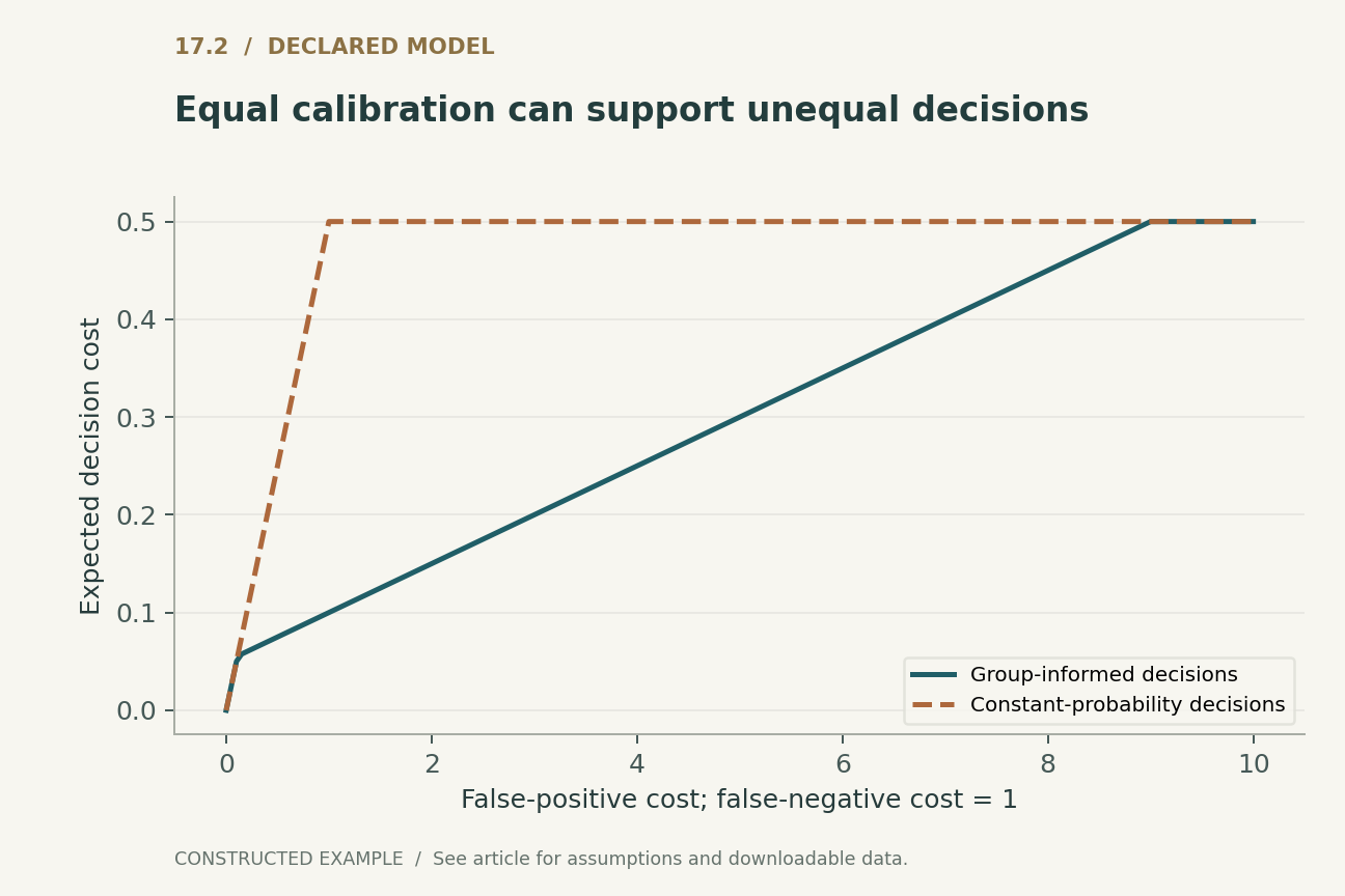
Suppose action one incurs cost C_FP when the event is absent, while action zero incurs cost C_FN when it is present. If p is the true event probability conditional on the information used, the expected costs are C_FP times one minus p and C_FN times p. Choose action one when p exceeds C_FP divided by the sum of the two costs; ties can be resolved by either action without changing expected cost.
With equal costs, the constant forecast cannot distinguish our two groups and incurs error one half. Using their conditional probabilities yields error one tenth. The second figure varies the false-positive cost while holding the false-negative cost at one. It compares decisions based on the constant information set with decisions based on group information. Both forecasts are calibrated relative to what they reveal, yet their attainable costs differ. This is an information comparison, not evidence that a specific neural calibrator achieves such gains.
7. Multiclass flexibility must pay its estimation cost
Kull and colleagues introduce Dirichlet calibration, which transforms log probabilities through a learned linear map and softmax. Compared with a single temperature, this allows class-specific corrections and interactions among probability coordinates. Their work is a multiclass calibration method, not a guarantee that additional flexibility always improves held-out reliability.
The extra parameters create an ordinary estimation problem. A small calibration set may not identify a useful correction for rare classes, and unconstrained flexibility can fit sampling noise. Regularization, class support, and separate evaluation data therefore belong in the method description. Changing the highest-probability class can improve or worsen classification; unlike a common positive temperature, a general map need not preserve rankings. Any downstream workflow that assumed unchanged decisions must be retested. Calibration training should also be isolated from repeated test-set tuning, since selecting a map on the same examples used for its final reliability diagram biases the apparent result. [3]
8. Selection and shift change the relevant population
A probability statement is indexed by a population. If a service routes low-confidence cases to a human, the retained distribution differs from the original test set. Calibration conditional only on the reported score survives selection determined solely by that score, provided the selection mechanism introduces no further outcome information. It need not survive selection that also uses an unmodeled subgroup, acquisition channel, or hidden difficulty signal. Stating the selection rule makes this distinction testable.
A changed class prevalence can also alter the interpretation of a fixed score. Recalibrating after every detected input shift is not automatically justified: an input change need not change the conditional outcome mechanism, and lack of input change does not exclude a label change. The deployment record should distinguish an alarm about distributional difference from evidence of probability error. Delayed labels, missing outcomes, and selective feedback complicate that evidence and should remain visible in reliability dashboards.
9. What the executed finite checks establish
The accompanying code represents twenty equally weighted cases: ten in each constructed group, with one and nine positive outcomes respectively. It verifies the constant forecast's aggregate calibration, its subgroup discrepancies, and the exact Brier losses of the constant and informative forecasts. A separate bin-merging example verifies that a coarser grouping can suppress an error statistic. All frequencies are deliberately assigned; they are not estimates from an external dataset.
For the cost sweep, exact conditional expectations select the lower-cost action independently in each information group. The checks compare these decisions with direct enumeration over the finite outcomes at selected costs. The temperature check confirms ordering preservation for representative non-tied logits and positive temperatures. These tests catch algebra, implementation, and figure mismatches. They cannot validate calibration on real users or demonstrate that a postprocessing method generalizes from a finite validation set. That latter claim requires the proposed held-out study.
10. Build an evaluation around decisions and uncertainty
A practical calibration report should begin with the output probability being interpreted and the decision it will inform. It should then provide a proper scoring rule, explicit reliability conditioning, uncertainty intervals, and decision costs or a justified range of costs. Coverage after abstention and class-specific support belong beside the headline metric. A comparison is stronger when it shows the same held-out population before and after a calibration map, including cases where performance worsens.
The resulting standard is demanding but concrete. Aggregate calibration is a useful constraint, not a complete objective. Flexible correction can improve a misspecified probability map, but must be estimated and evaluated separately. Better probability information can reduce decision cost even when both competing forecasts satisfy a calibration statement. These are analytical conclusions supported by the disclosed constructions. The article proposes, but has not run, a neural calibration trial across acquisition domains, class prevalences, and operational thresholds.
Executed locally · Bounded scope
Calibrated-but-uninformative population, bin merging, and cost-optimal actions
Assigned finite outcomes and population expectations; binary event-probability bins, not multiclass confidence ECE. No validation-set fitting or real-user outcomes.
516 assertions passed. These checks validate the supplied example, not the cited systems.
Inspect the recorded witness
{
  "cases": 20,
  "group_positive_counts": [
    1,
    9
  ],
  "constant_Brier": 0.25,
  "informed_Brier": 0.09,
  "coarse_probability_ECE": 0.0,
  "fine_probability_ECE": 0.25,
  "cost_at_equal_error_costs": {
    "pooled": 0.5,
    "informed": 0.1
  }
}
Example runner · Model loader · Training models · Representation models · Generation models · Reliability modelsRead the complete check results
A declared analytical model
Four equations, explicit assumptions
(1) Positive temperature scaling preserves logit order; a temperature is fitted on separate calibration data and evaluated on untouched examples.
(2) Population bin-based event-probability calibration error for binary Y. It is not automatically the conventional selected-class confidence ECE; bins are part of the definition.
(3) For fixed p and Bernoulli Y with probability q. In the constructed groups q is 0.1 or 0.9; Brier loss is 0.09+0.16(1-alpha)^2 under the stated interpolation.
(4) Binary action with nonnegative error costs and a positive sum; p must represent the conditional event probability for the information available to the decision.
Constructed examples · Reproducible data
Inspect the quantitative argument
These curves are calculated from the declared models. They are not observations from the cited studies. Every figure includes its numeric data and vector version.


Which evidence answers which question?
| Evaluation | Useful question | Blind spot |
|---|---|---|
| Top-class confidence | How often is the selected class correct at this confidence? | Other coordinates of the probability vector |
| Classwise reliability | Does each class probability match its event frequency? | All possible joint or subgroup conditions |
| Brier or log score | Are informative accurate probabilities rewarded? | Which subgroup accounts for an aggregate error |
| Expected action cost | Does the probability support this decision? | Other decisions with different costs |
A proposed validation protocol
This is a proposed evaluation design. No production-system or hardware benchmark was performed. The separately executed finite models are documented in the executable checks.
- Freeze the probability target, action space, cost range, and deployment population.
- Separate model training, calibration fitting, method selection, and final evaluation examples.
- Compare uncalibrated predictions, a positive temperature baseline, and a regularized flexible map.
- Report proper scores and reliability curves with explicit bin rules, support counts, and uncertainty.
- Evaluate subgroup and selected-population reliability without hiding abstentions or rare classes.
- Measure cost and coverage under prespecified thresholds, then repeat on genuinely held-out shifts.
What the primary sources establish
Chuan Guo, Geoff Pleiss, Yu Sun et al. · 2017 [1]
Contribution. Studies neural-network miscalibration and temperature scaling as a postprocessing method.
Boundary. Empirical effectiveness is dataset-dependent; temperature preserves class order.
Source locator. Sections 2 and 4, temperature scaling.
Juozas Vaicenavicius, David Widmann, Carl Andersson et al. · 2019 [2]
Contribution. Formalizes different probabilistic calibration notions and their evaluation.
Boundary. A scalar summary does not characterize every conditioning event.
Source locator. Sections on calibration definitions and evaluation.
Meelis Kull, Miquel Perello-Nieto, Markus Kängsepp et al. · 2019 [3]
Contribution. Introduces a multiclass calibration map based on log probabilities and a linear-softmax transformation.
Boundary. Additional expressivity requires adequate fitting and independent evaluation.
Source locator. Dirichlet calibration definition and parameterizations.
Limits of this analysis
- The twenty-case population is constructed and is not evidence about any real subgroup.
- Exact population calculations avoid sampling noise that a real calibration study must quantify.
- Three foundational sources do not constitute an exhaustive comparison of modern calibration methods.
- The cost model assumes binary actions and known costs; complex decisions need their own utility model.
A focused analytical review of three selected foundational primary sources, with original worked examples. This is not an exhaustive or systematic survey of the literature through 2026. Source access and version notes are recorded with the bibliography.
Questions that would change the conclusion
- Which calibration conditioning events are necessary for a particular downstream decision?
- How can rare-group reliability be estimated without hiding its statistical uncertainty?
- When does a flexible multiclass map improve expected decision cost beyond a well-fitted scalar temperature?
References
- Chuan Guo, Geoff Pleiss, Yu Sun et al.. On Calibration of Modern Neural Networks. Proceedings of the 34th International Conference on Machine Learning (2017). Primary source.
- Juozas Vaicenavicius, David Widmann, Carl Andersson et al.. Evaluating model calibration in classification. Proceedings of the Twenty-Second International Conference on Artificial Intelligence and Statistics (2019). Primary source.
- Meelis Kull, Miquel Perello-Nieto, Markus Kängsepp et al.. Beyond temperature scaling: Obtaining well-calibrated multiclass probabilities with Dirichlet calibration. Advances in Neural Information Processing Systems 32 (2019). Primary source.
Source [1] access. Primary record and selected accessible full-text sections inspected; no exhaustive supplementary-material audit.
Source [2] access. Primary record and selected accessible full-text sections inspected; no exhaustive supplementary-material audit.
Source [3] access. Primary record and selected accessible full-text sections inspected; no exhaustive supplementary-material audit.
Bibliographic identities were checked against primary publisher and author records. Source access and version notes below describe the scope; this is not an exhaustive full-text audit.
Authorship and provenance
Written and technically self-reviewed by Codex (AI). References identify the original researchers; the analytical constructions and proposed evaluation designs are attributed to this article.
Covers are conceptual ImageGen illustrations. Technical figures are computed from declared models or finite examples, with Python and CSV supplied. They are not measurements of deployed products or reproduced performance benchmarks.
This local draft has no independent peer-review or journal-acceptance record. Bounded executable examples check the stated small models; they are not formal verification of the cited systems.