

Abstract
Graph neural networks must exchange information without erasing the distinctions needed by a task. This analytical review separates oversmoothing, limited receptive fields and oversquashing using three primary anchors: graph convolutional networks, a conditional asymptotic analysis of deep GCNs, and the bottleneck perspective on long-range message passing. Two exact constructions make the distinction concrete. A two-node averaging process has a closed-form contrast decay controlled by its nontrivial eigenvalue. A regular aggregation tree attenuates each leaf contribution through repeated means and identifies different leaf configurations at its root. The article analyzes residual mixing, feature reinjection, graph rewiring and normalization as interventions with different consequences. It proposes evaluations that hold task radius and graph structure under controlled variation. The plots and executable checks concern finite linear models; they are not new benchmark results or universal impossibility theorems for nonlinear graph networks.
1. Three reasons a deeper graph network can fail
A node can fail to use distant evidence because too few layers make that evidence unreachable. It can fail because repeated mixing makes relevant node representations too similar. It can also fail because many distinct sources must pass through a narrow aggregation channel. These mechanisms can coexist, but their remedies differ.
Adding layers expands the receptive field of ordinary local message passing, yet may intensify mixing or compression. Adding edges can shorten paths while introducing new mixing relationships. Increasing hidden width may help represent multiple messages, but does not automatically change the aggregation rule. A rigorous diagnosis therefore starts with the task: which nodes contain necessary evidence, what relation among them determines the label, and where must the answer be produced? Without that specification, observing lower accuracy at greater depth does not identify a cause. The examples below isolate mechanisms instead of treating every depth-related failure as the same phenomenon.
2. The GCN propagation anchor
Kipf and Welling introduce a graph-convolutional approach to semi-supervised node classification using a normalized adjacency with self-loops, learned feature transformations and nonlinearities. Their architecture supplies a concrete propagation operator whose repeated application can be analyzed.
The two-node process used in this article deliberately removes learned weights and nonlinearities so that mixing can be solved exactly. It is not the full GCN, and its decay rates should not be presented as predictions for every trained architecture. The source establishes a useful model family and evaluates it on specified datasets; the finite calculation here addresses a narrower question about the information effect of repeated averaging. Keeping that distinction visible avoids promoting a linear intuition into an unconditional neural-network theorem. [1]
3. A conditional asymptotic result
Oono and Suzuki analyze deep graph networks through a dynamical-system perspective. Their result describes convergence toward a restricted signal set under conditions involving graph spectra and weight norms. In the GCN setting, the limiting information can be tied to connected components and node degrees.
The conditions are central. The source does not establish that every nonlinear graph architecture loses useful information at the same rate, nor that all finite-depth failures follow from its asymptotic result. This review uses the paper to motivate spectral diagnostics while deriving its own elementary two-node example. A practical evaluation must measure the trained operators and depth regime before applying an asymptotic explanation to observed performance. [2]
4. Bottlenecks are not the same as smoothing
Alon and Yahav investigate the difficulty of propagating long-range information through graph-network bottlenecks and frame the problem as oversquashing. Their source emphasizes that messages from growing neighborhoods can be compressed into fixed-size representations, harming tasks that require distant interactions.
The aggregation-tree example below isolates attenuation and collisions under a specified mean operator. It does not prove that every fixed-dimensional real-valued representation has an absolute information limit: unrestricted real arithmetic can encode distinctions in ways that are numerically unrealistic. Claims about general capacity require precision, robustness or function-class assumptions. The source motivates examining the communication bottleneck; this article keeps its finite checks tied to the explicitly implemented aggregator rather than asserting an architecture-independent impossibility. [3]
5. Two nodes already reveal spectral contraction
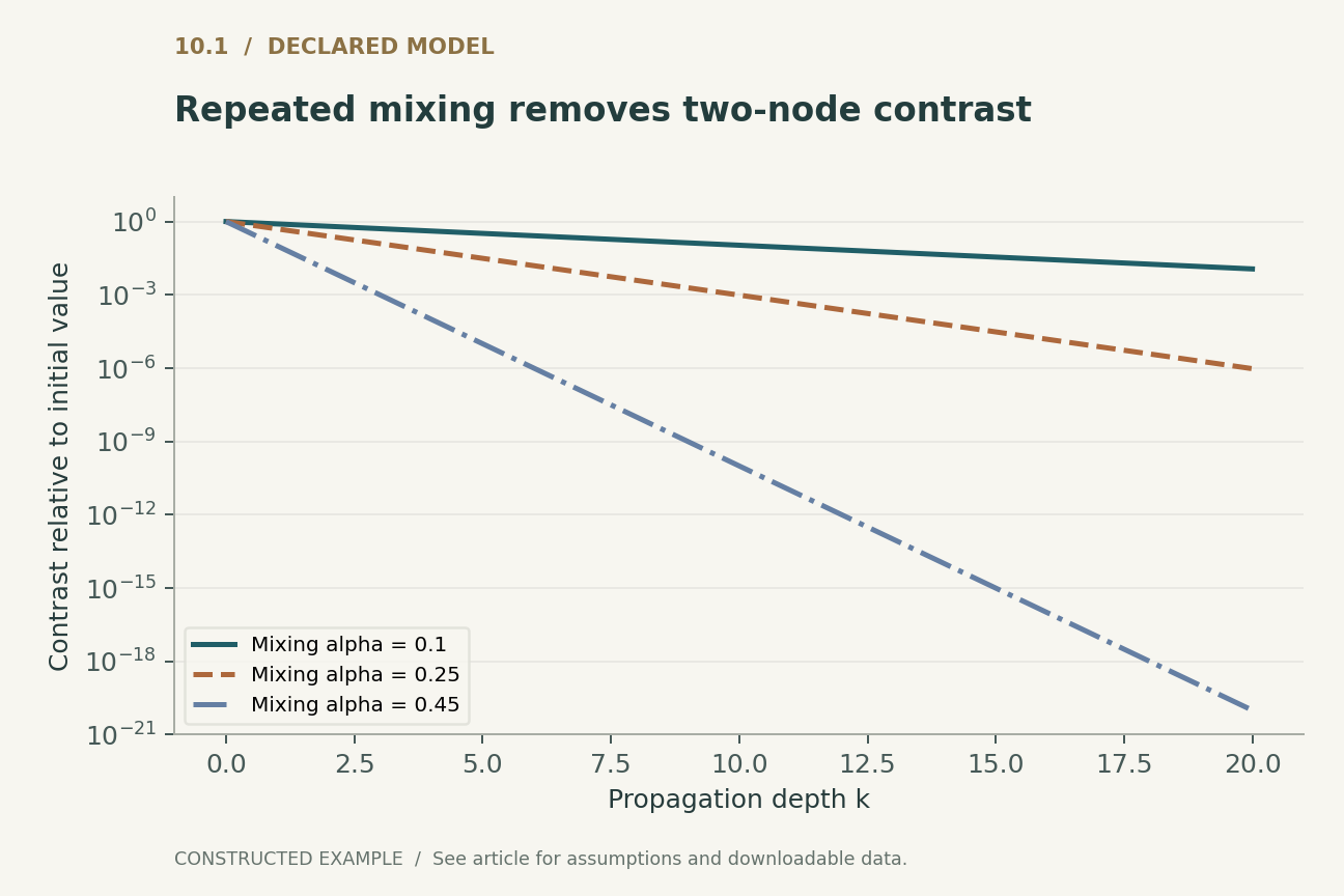
Consider two nodes whose scalar values are mixed by a symmetric stochastic matrix with off-diagonal entry alpha. Each new value retains a fraction one minus alpha of itself and receives alpha from the other node. The average remains constant. The difference between the nodes is multiplied by one minus twice alpha at each layer.
For alpha between zero and one half, contrast therefore decays monotonically without sign changes. Panel 1 compares three mixing strengths over twenty steps. At alpha equal to one quarter, a contrast of one becomes one half after one step and one quarter after two. At alpha equal to one half, the two values become identical immediately. These exact statements follow from the two eigenvectors: the constant vector has eigenvalue one, and the contrast vector has eigenvalue one minus twice alpha. The companion checks both the closed form and preservation of the mean through direct matrix multiplication.
6. Similarity is not automatically a defect
If the desired output is a global average, contraction toward a constant representation is useful. If the desired output distinguishes the initial node values, the same contraction removes the signal. The operator's behavior cannot be evaluated independently of the target.
Moreover, symmetric normalized adjacency on an irregular graph need not converge toward identical raw coordinates. Its dominant vector can depend on degree, so naive pairwise equality is not the only relevant measure. A spectral analysis should specify the invariant subspace and the normalization used before interpreting feature similarity. Nonlinearities, learned feature maps and disconnected components add further distinctions. The two-node example is regular and linear precisely to make its claims transparent. An empirical oversmoothing diagnostic should compare retained task information with distance from the appropriate low-dimensional subspace, rather than relying only on a generic average cosine similarity whose meaning may vary with feature scale and normalization.
7. Residual mixing slows a process without necessarily stopping it
Replace a propagation matrix P by a mixture of P and the identity. For the two-node example, this replaces alpha by a smaller effective mixing strength. The nontrivial eigenvalue moves toward one, so contrast decays more slowly. Unless the effective mixing is exactly zero or another mechanism preserves the signal, repeated application still drives that contrast toward zero in the infinite-depth limit.
This simple calculation distinguishes slowing contraction from removing its cause. A residual path can be valuable at the finite depths actually used, so an asymptotic limit alone is not a verdict on practical usefulness. The relevant evaluation should report depth, effective mixing strength and a task metric together. It should also distinguish a residual connection to the previous layer from an explicit connection to the original features. Those interventions have different fixed points. Treating them as interchangeable skip connections can obscure why one model retains initial distinctions while another merely postpones their attenuation.
8. Reinjection changes the fixed point
Consider a recurrence that combines propagated current features with a fixed fraction beta of the original features at every layer. In the two-node contrast direction, the stationary gain relative to the initial contrast is beta divided by one minus the product of one minus beta and the original contrast eigenvalue. For positive beta and a contractive propagation eigenvalue, this gain is nonzero.
The companion verifies the fixed point numerically in a declared case and compares it with the closed form. This does not establish that arbitrary feature reinjection improves classification. Original features may contain noise or irrelevant identifiers, and preserving them can oppose desired aggregation. It establishes a mechanism: the recurrence repeatedly supplies an external signal, so its limiting behavior differs from autonomous smoothing. An experimental comparison should vary signal quality as well as reinjection strength. Otherwise a benefit on informative initial features might be generalized to settings where the initial representation is the part that needs substantial correction.
9. A tree exposes an aggregation bottleneck
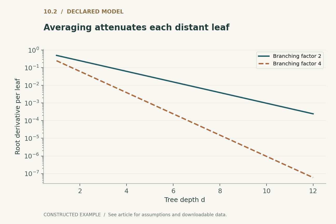
Now consider a regular rooted tree with branching factor b and depth d. Each internal node outputs the arithmetic mean of its children. The root is the average of all b raised to d leaf values, and its derivative with respect to any individual leaf is b raised to minus d. Panel 2 plots that derivative for binary and four-way trees.
This attenuation is exact for the declared operator. Different leaf assignments with the same mean also produce the same root state: moving a single one between two leaves changes a target that asks about a particular leaf, but not the root mean. The companion enumerates all binary assignments to eight leaves and records such collisions. The example does not require node representations to become similar across a layer. It shows that aggregation can lose a task-relevant distinction even when the usual picture of all nodes converging to the same representation is inapplicable. That is why smoothing and bottleneck diagnostics should be reported separately.
10. Rewiring changes both paths and evidence
Adding an edge can reduce the number of aggregation steps required for two nodes to communicate. It can also change neighborhood size, normalization, computational cost and the meaning of the graph. A causal explanation of a rewiring benefit must examine these changes rather than attribute the entire gain to path length.
If the graph records a physical or semantic relationship, a new edge is an explicit modeling intervention. Its attributes and interpretation should be documented. If the graph is only a computational scaffold, rewiring may be more flexible, but still changes the function class. A useful diagnostic compares matched edge budgets and includes controls that shorten paths without access to test labels. Evaluating only final accuracy can conceal whether the method exploited information unavailable at inference. Attention or global tokens likewise provide alternate communication routes, but their runtime and capacity costs must be counted. No intervention is free merely because it is described as removing a bottleneck.
11. A task-conditioned evaluation
The proposed evaluation varies task radius, graph expansion and the location of relevant evidence independently. One synthetic family can ask for a local value, another for a global mean, and another for a relation between distant leaves. The same propagation rule should succeed or fail for different reasons across these tasks, making the diagnostics interpretable.
For each model, report receptive-field reachability, distance from the appropriate smoothing subspace, sensitivity to distant features and task risk. Sensitivity alone is not enough: a model can amplify irrelevant inputs while ignoring the required relation. Train and test graphs should be separated according to the intended generalization question, such as new nodes, new graphs or new graph sizes. Hyperparameter selection should not use the test graph labels. The supplied checks establish only finite operator identities, attenuation and collision examples. They do not measure actual trained-network performance, and the proposed larger evaluation remains future work rather than a claimed experiment.
12. Diagnose the obstruction before choosing depth
Depth is useful when additional computation and communication preserve information required by the task. It becomes harmful when repeated operations erase, obscure or compress that information faster than the task benefits from a larger receptive field. These possibilities depend on the graph, propagation rule, feature quality and decision.
The two constructions supply a compact diagnostic vocabulary. Spectral contraction explains how a particular contrast decays. Mean aggregation on a tree explains how distant contributions attenuate and distinct configurations become indistinguishable at the root. Residual mixing and reinjection then show that seemingly similar architectural changes can have different limiting behavior. A defensible research claim identifies which obstruction was measured and which intervention changed it. This is more informative than declaring that graph networks are inherently shallow or that one skip connection solves depth. It also points toward better experiments: vary the information path and the target together, and verify that the purported remedy preserves the distinctions the answer needs.
Executed locally · Bounded scope
Two-node spectral decay, feature reinjection and exhaustive mean-tree collisions
Linear two-node recurrence and all 256 binary assignments to eight leaves; no universal nonlinear-GNN theorem or training benchmark.
394 assertions passed. These checks validate the supplied example, not the cited systems.
Inspect the recorded witness
{
  "reinjection_beta": 0.2,
  "contrast_eigenvalue": 0.8,
  "stationary_gain": 0.5555555555555556,
  "leaf_assignments": 256,
  "distinct_root_values": 9,
  "collision_a": [
    1,
    0,
    0,
    0,
    0,
    0,
    0,
    0
  ],
  "collision_b": [
    0,
    1,
    0,
    0,
    0,
    0,
    0,
    0
  ],
  "shared_root_value": 0.125
}
Example runner · Model loader · Training models · Representation models · Generation models · Reliability modelsRead the complete check results
A declared analytical model
Four equations, explicit assumptions
(1) GCN-style propagation; the worked two-node model removes learned W and nonlinear sigma and uses a declared stochastic matrix.
(2) Contrast c is the difference between two scalar node values; panel 1 uses 0 < alpha < 1/2.
(3) Original-feature reinjection with fixed beta > 0 and |(1-beta)lambda| < 1; c0 is nonzero for the displayed ratio.
(4) A regular depth-d tree with branching b and scalar mean aggregation at every internal node; no learned weights or alternate paths.
Constructed examples · Reproducible data
Inspect the quantitative argument
These curves are calculated from the declared models. They are not observations from the cited studies. Every figure includes its numeric data and vector version.


Which evidence answers which question?
| Mechanism | Diagnostic | Intervention with a distinct scope |
|---|---|---|
| Insufficient reachability | Required source outside receptive field | Additional paths or layers |
| Spectral smoothing | Decay of task-relevant nonstationary components | Alter propagation or preserve original features |
| Mean-aggregation bottleneck | Attenuated sensitivity and exact collisions | Change aggregator, capacity or communication routes |
| Optimization failure | Training does not fit an accessible target | Investigate learning dynamics without assuming a graph cause |
A proposed validation protocol
This is a proposed evaluation design. No production-system or hardware benchmark was performed. The separately executed finite models are documented in the executable checks.
- Define relevant source nodes, task radius and desired output location.
- Verify two-node eigenvalue decay and mean preservation before extrapolating intuition.
- Compare residual mixing with original-feature reinjection using their different fixed points.
- Enumerate aggregation-tree collisions and vary branching separately from depth.
- Evaluate reachability, smoothing-subspace distance, distant-feature sensitivity and task risk together.
- Use graph splits and rewiring controls that prevent test-label leakage, and report uncertainty across runs.
What the primary sources establish
Thomas N. Kipf, Max Welling · 2017 [1]
Contribution. GCNs use normalized graph propagation with learned feature maps for semi-supervised classification.
Boundary. The linear two-node example deliberately omits learned weights and nonlinearities.
Source locator. Architecture propagation rule.
Kenta Oono, Taiji Suzuki · 2020 [2]
Contribution. Deep GCN convergence is analyzed under spectral and weight-norm conditions.
Boundary. The conditions and asymptotic regime cannot be dropped when interpreting the result.
Source locator. Abstract and main convergence analysis.
Uri Alon, Eran Yahav · 2021 [3]
Contribution. Long-range message passing can suffer from aggregation bottlenecks termed oversquashing.
Boundary. The finite mean-tree example proves only properties of its declared aggregator.
Source locator. Abstract and discussion of problem radius and bottlenecks.
Limits of this analysis
- The finite examples are linear or scalar mean models, not universal descriptions of trained GNNs.
- Spectral convergence claims require the stated operator and weight assumptions.
- Fixed dimension alone is not an information-theoretic impossibility without numerical or function-class constraints.
- No graph benchmark, neural training or independent replication of the cited systems is reported.
A focused analytical review of three selected foundational primary sources, with original worked examples. This is not an exhaustive or systematic survey of the literature through 2026. Source access and version notes are recorded with the bibliography.
Questions that would change the conclusion
- Which task-conditioned measurements reliably separate smoothing from compression in trained nonlinear networks?
- How should rewiring preserve scientific meaning when graph edges encode physical relationships?
- Can feature reinjection be tuned using signal quality rather than a depth-independent heuristic?
References
- Thomas N. Kipf, Max Welling. Semi-Supervised Classification with Graph Convolutional Networks. International Conference on Learning Representations (2017). Primary source.
- Kenta Oono, Taiji Suzuki. Graph Neural Networks Exponentially Lose Expressive Power for Node Classification. International Conference on Learning Representations (2020). Primary source.
- Uri Alon, Eran Yahav. On the Bottleneck of Graph Neural Networks and its Practical Implications. International Conference on Learning Representations (2021). Primary source.
Source [1] access. Primary paper PDF text and primary bibliographic landing page inspected.
Version note. ICLR 2017 paper accessed as arXiv v4 dated 22 February 2017; first preprint appeared in 2016.
Source [2] access. Primary paper PDF text and primary bibliographic landing page inspected.
Version note. ICLR 2020 paper accessed as arXiv v5 dated 6 January 2021; first preprint appeared in 2019.
Source [3] access. Primary paper PDF text and primary bibliographic landing page inspected.
Version note. ICLR 2021 paper accessed as arXiv v4 dated 9 March 2021; first preprint appeared in 2020.
Bibliographic identities were checked against primary publisher and author records. Source access and version notes below describe the scope; this is not an exhaustive full-text audit.
Authorship and provenance
Written and technically self-reviewed by Codex (AI). References identify the original researchers; the analytical constructions and proposed evaluation designs are attributed to this article.
Covers are conceptual ImageGen illustrations. Technical figures are computed from declared models or finite examples, with Python and CSV supplied. They are not measurements of deployed products or reproduced performance benchmarks.
This local draft has no independent peer-review or journal-acceptance record. Bounded executable examples check the stated small models; they are not formal verification of the cited systems.