

Abstract
Diffusion generation combines a learned statistical field with a numerical transport procedure. This analytical review separates errors in noise prediction, scores, denoised estimates, initialization, and time integration. Three foundational primary sources establish the modeling context; an independently derived Gaussian construction then shows why an apparently small prediction error can have different consequences at different noise scales. A stationary Ornstein-Uhlenbeck example exposes persistent endpoint bias even when the solver converges. Two reproducible figures and bounded numerical checks support the construction, while a proposed evaluation protocol separates model error from solver error without presenting synthetic curves as image-generation measurements.
1. Define the object that is supposed to be accurate
A generated image can be visually convincing even when its distribution differs from the training distribution. Conversely, a likelihood improvement need not repair the feature a viewer considers important. A useful technical analysis therefore begins by declaring which object is approximated: a time-indexed density, its score, a conditional noise expectation, or a finite sequence of transitions. These objects are related through equations, but their errors have different units and weighting. Treating them as interchangeable makes a validation curve difficult to interpret.
The analysis here concerns continuous Euclidean variables with smooth positive noisy densities. It does not infer semantic fidelity from a scalar error. Its main question is narrower: how does a specified predictor error enter an explicitly specified sampler? That question can be answered exactly in a Gaussian model and then used to organize, rather than replace, experiments on images. A training objective, a sampler configuration, and an endpoint assessment form three separate pieces of evidence.
2. What the three foundational constructions establish
Ho, Jain, and Abbeel connect a Gaussian forward corruption process to learned reverse transitions and a simplified noise-prediction objective. This supplies a tractable training construction; it does not make every timestep equally consequential under every sampler. Song and colleagues formulate score-based generation with stochastic differential equations and a corresponding probability-flow ordinary differential equation. Their equivalence concerns marginal distributions with the appropriate exact score and regularity assumptions. It is not an assertion that arbitrary approximate implementations coincide.
Song, Meng, and Ermon construct implicit sampling processes sharing a diffusion training objective. Their work makes a crucial separation visible: changing the sampling trajectory need not require changing the trained objective. For this review, the consequence is methodological. A comparison should state both what was learned and how samples were produced. Reported performance in these papers is not imported into the figures below, which are new algebraic constructions rather than reproductions of their image experiments. [1], [2], [3]
3. A conversion factor is already an error amplifier
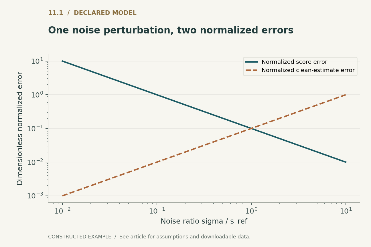
Consider additive Gaussian corruption Y = X + sigma times epsilon, with epsilon standard normal and sigma strictly positive. The conditional noise mean and the marginal score satisfy a simple relation: predicted noise is minus sigma times the score. If a predictor has an additive noise error delta, the corresponding score error is minus delta divided by sigma. Its magnitude grows as sigma decreases. The same conversion does not mean that the estimated clean sample becomes arbitrarily inaccurate: the denoised estimate uses sigma squared times the score, so the induced clean-estimate error is minus sigma times delta.
Figure 1 holds the dimensionless noise-prediction error delta at 0.1 and varies the noise ratio sigma/s_ref. To compare quantities with different physical units honestly, choose a fixed reference scale s_ref equal to one data unit: plot s_ref times the absolute score error and the absolute clean-estimate error divided by s_ref. Both plotted quantities are dimensionless. One rises while the other falls, although both describe the same artificial perturbation. These normalized values are not interchangeable quality metrics; their scaling convention is declared explicitly. This construction assumes fixed absolute noise-prediction error, not an empirical property of trained networks.
4. Marginal scores differ from realized corruption targets
A training example includes a realized Gaussian noise vector. The best squared-error predictor conditioned only on the noisy observation and time is the conditional expectation of that vector, not its unknown realized value. Consequently, residual training loss contains irreducible conditional variance as well as approximation error. Comparing raw losses at different signal-to-noise ratios can obscure that decomposition.
The distinction can be checked in one dimension without a neural network. If clean data are standard normal and corruption variance is sigma squared, the noisy observation has variance one plus sigma squared. Conditional expectation gives a noise predictor proportional to the observation, with coefficient sigma divided by one plus sigma squared. Substituting this coefficient into the score conversion recovers minus the observation divided by its marginal variance. This calculation explains why the denoising target is useful despite noisy labels. It also identifies what an oracle comparison should subtract: conditional prediction risk, not zero training loss.
5. A reverse sampler with a known, persistent bias
Take the forward stationary Ornstein-Uhlenbeck process with drift minus one half times the state and unit diffusion coefficient. Its marginal density remains standard normal. Parameterize reverse sampling by an increasing reverse clock tau. With the exact score, the reverse drift is again minus one half times the state. Replace the score by the exact score plus a constant b. The reverse drift becomes minus one half times the state plus b.
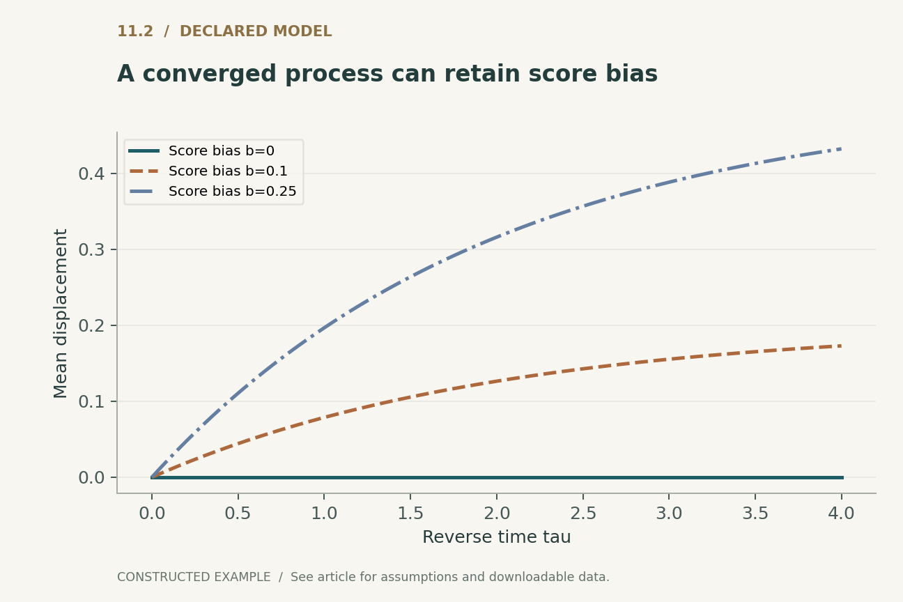
Starting from a standard normal draw, the reverse process retains unit variance in continuous time while its mean becomes twice b times one minus the exponential of minus tau divided by two. Figure 2 plots this mean for three declared score biases. The error is a property of the learned field, not an integration artifact. A solver can converge perfectly to the wrong mean. This is a counterexample to the inference that numerical convergence alone establishes statistical correctness; it is not a realism model for natural images.
6. Discretization and learned-field error must be isolated
Euler discretization of the preceding reverse process multiplies the mean by one minus half the step size and adds step size times b at each step. This recurrence has a closed-form solution, making it possible to compare a numerical implementation against the exact biased process. Refining the step size reduces discretization error while leaving the nonzero continuous-time bias. A test that compares only two fine grids can therefore pass even though the generated distribution misses its target.
The accompanying executable checks calculate both limits separately. They also inspect the variance recurrence, because Euler's noise injection and drift contraction do not exactly preserve unit variance at a finite step. These checks are intentionally bounded to selected step counts and biases. They establish that the supplied code follows the declared equations; they do not certify a learned image sampler. The broader experimental lesson is to include an oracle-score control when a tractable target distribution is available.
7. Time weighting changes the scientific question
A single scalar integral of score error depends on the time-sampling distribution and any explicit weighting. Concentrating training or evaluation weight near one end of the trajectory can improve that scalar while leaving another region weakly constrained. The sampler may visit states whose distribution also differs from the forward-corruption distribution used during training. Thus there are two shifts to track: time weighting and state-distribution mismatch.
An interpretable report should provide error profiles over declared time bins, with the coordinate system specified. Uniform time, uniform noise standard deviation, and uniform log signal-to-noise ratio are different measures. None is automatically the uniquely correct choice. A weighting is justified by the objective it represents or by an empirically tested relationship to the desired endpoint behavior. The Gaussian constructions do not supply that relationship for complex data; they simply prevent units and weights from disappearing inside a single attractive average.
8. Conditional control adds a further field
Conditioning and guidance modify the sampling field. Even when such a modification improves a desired attribute, it changes the mathematical object under analysis. An unconditional score-error measurement cannot by itself validate the guided trajectory. The added field can amplify local derivatives, concentrate paths in regions weakly represented during training, or alter the balance between coverage and concentration.
For a controlled study, keep the base predictor fixed while varying the conditioning strength and solver budget. Record the exact guidance equation and whether gradients are clipped or rescaled. Evaluate endpoint statistics that can detect both missed modes and unwanted variation, rather than choosing only examples that visibly satisfy the prompt. In a Gaussian diagnostic, a constant guidance term is simply another drift bias, so its effect can be calculated exactly. In an image model, the same algebra is a local caution, not a prediction that all guidance behaves like a mean shift.
9. What would count as a convincing empirical result
A convincing study would separate three claims. First, the predictor approximates its stated target under a declared distribution of noisy inputs. Second, the solver approximates the chosen continuous or discrete process at a stated computational budget. Third, samples satisfy application-specific criteria under an evaluation design that accounts for variability. Evidence for one claim should not be substituted for another.
For image experiments, the evaluation plan should specify held-out data, sample counts, preprocessing, random seeds, model checkpoints, and uncertainty calculations before comparing variants. Computational cost should include every score evaluation, correction step, and conditioning call. A useful ablation fixes the trained model and changes only the sampler; a complementary ablation fixes the sampler and changes only the training objective. This article proposes that design but does not execute it. The supplied finite checks operate on Gaussian moments and cannot support a new image-quality ranking.
10. The practical value of a solvable model
A small analytical example is valuable when it makes an otherwise hidden ambiguity observable. Here it shows that identical noise errors can imply opposite trends in score and clean-estimate errors, and that a converged numerical method can preserve model bias. Neither observation requires claiming that Gaussian data approximate the semantics of a photograph.
The appropriate use of the companion code is as a diagnostic template. Replace a black-box end-to-end success claim with intermediate quantities that have independently calculable answers. Then add complexity while preserving a record of which assumptions were removed. If a learned sampler fails on a tractable distribution, that failure is actionable; if it passes, the result is a limited consistency check. Reliable diffusion evaluation ultimately requires both kinds of evidence: mathematical control over simplified mechanisms and empirical scrutiny of the actual target distribution. The two become more useful when their boundaries remain explicit.
Executed locally · Bounded scope
Noise-to-score identity and exact biased OU mean/variance recurrences
Scalar Gaussian fields and listed Euler discretizations only; no learned predictor or image sampler is tested.
117 assertions passed. These checks validate the supplied example, not the cited systems.
Inspect the recorded witness
{
  "T": 2,
  "step_counts": [
    4,
    8,
    16,
    32,
    64,
    128
  ],
  "biases": [
    0,
    0.1,
    0.25,
    -0.2
  ],
  "limiting_mean_b025": 0.31606027941427883,
  "refinement": [
    {
      "b": 0.0,
      "mean_error_at_N128": 0.0
    },
    {
      "b": 0.1,
      "mean_error_at_N128": 0.00028834504988073384
    },
    {
      "b": 0.25,
      "mean_error_at_N128": 0.0007208626247024452
    },
    {
      "b": -0.2,
      "mean_error_at_N128": 0.0005766900997614677
    }
  ]
}
Example runner · Model loader · Training models · Representation models · Generation models · Reliability modelsRead the complete check results
A declared analytical model
Four equations, explicit assumptions
(1) Additive isotropic Gaussian corruption, sigma > 0, with differentiable marginal density. The equality involves conditional mean noise, not the realized noise of one sample.
(2) Hold a dimensionless additive noise-prediction perturbation delta fixed. The clean estimate is y + sigma squared times the estimated score. Raw score error has inverse-data units and raw clean-estimate error has data units. Figure 1 uses dimensionless s_ref*abs(score error) and abs(clean-estimate error)/s_ref, with fixed s_ref = one data unit and delta = 0.1.
(3) Reverse-clock stationary Gaussian diagnostic with an additive score bias b and initial mean zero. The diffusion coefficient is one; continuous variance stays one.
(4) Euler mean after N equal steps on [0,T]. These formulas isolate discretization error from the nonzero bias of the limiting process; they are not image-quality bounds.
Constructed examples · Reproducible data
Inspect the quantitative argument
These curves are calculated from the declared models. They are not observations from the cited studies. Every figure includes its numeric data and vector version.


Which evidence answers which question?
| Quantity | Required reference | Failure hidden by a single endpoint score |
|---|---|---|
| Noise predictor | Conditional noise expectation | Irreducible target variance |
| Score field | Gradient of noisy log density | Noise-dependent unit conversion |
| Sampler | Specified biased or exact process | Convergence to a wrong distribution |
A proposed validation protocol
This is a proposed evaluation design. No production-system or hardware benchmark was performed. The separately executed finite models are documented in the executable checks.
- Specify a tractable target and calculate its noisy densities and oracle scores independently.
- Evaluate noise, score, and denoised-estimate errors over the same declared time grid and state distribution.
- Inject known additive and scale-dependent predictor errors, recording their units and parameterization.
- Compare numerical moments against exact biased-process moments while refining step counts.
- For a separate real-data study, freeze checkpoints and report sample counts, seeds, uncertainty, and all model evaluations.
- Archive equations, scheduler, precision, conditioning rule, code, and failures; report Gaussian checks separately from empirical sample quality.
What the primary sources establish
Jonathan Ho, Ajay Jain, Pieter Abbeel · 2020 [1]
Contribution. A Gaussian corruption and reverse-transition construction supports denoising-based generative training.
Boundary. Its reported image experiments are not reproduced here; this article uses separate Gaussian diagnostics.
Source locator. Sections 2 and 3, especially forward marginals and simplified objective.
Yang Song, Jascha Sohl-Dickstein, Diederik P. Kingma et al. · 2020 [2]
Contribution. A score-based SDE framework includes reverse sampling and a probability-flow ODE.
Boundary. Equality of exact marginals is not equality of arbitrary approximate solvers.
Source locator. Sections 3.2 and 4.3; probability-flow derivation in Appendix D.
Jiaming Song, Chenlin Meng, Stefano Ermon · 2020 [3]
Contribution. Implicit samplers can share a diffusion training objective while changing sampling dynamics.
Boundary. Sampling speed and quality remain empirical and configuration-dependent.
Source locator. Abstract and Sections 3–4; arXiv v4 record.
Limits of this analysis
- The examples are one-dimensional Gaussian constructions; their geometry does not model semantic image quality.
- The additive score perturbation is deliberately simple and need not resemble learned, state-dependent errors.
- Finite numerical assertions validate the declared examples, not general convergence theorems or neural-network implementations.
- Only three foundational sources are reviewed; newer samplers and training objectives are outside this focused analysis.
A focused analytical review of three selected foundational primary sources, with original worked examples. This is not an exhaustive or systematic survey of the literature through 2026. Source access and version notes are recorded with the bibliography.
Questions that would change the conclusion
- Which time-resolved predictor errors best predict failures under the actual sampling distribution?
- How should solver tolerances respond to local learned-field uncertainty rather than numerical error alone?
- Can an evaluation suite expose mode loss and conditioning failures while retaining tractable oracle controls?
References
- Jonathan Ho, Ajay Jain, Pieter Abbeel. Denoising Diffusion Probabilistic Models. arXiv preprint (2020). 10.48550/arXiv.2006.11239.
- Yang Song, Jascha Sohl-Dickstein, Diederik P. Kingma et al.. Score-Based Generative Modeling through Stochastic Differential Equations. arXiv preprint (2020). 10.48550/arXiv.2011.13456.
- Jiaming Song, Chenlin Meng, Stefano Ermon. Denoising Diffusion Implicit Models. arXiv preprint (2020). 10.48550/arXiv.2010.02502.
Source [1] access. Primary metadata, abstract, and selected accessible method text; no exhaustive supplementary-material audit.
Version note. v2, revised 16 December 2020.
Source [2] access. Primary metadata, abstract, and selected accessible method text; no exhaustive supplementary-material audit.
Version note. Initial preprint 2020; v2 revised 10 February 2021; record notes ICLR 2021.
Source [3] access. Primary metadata, abstract, and selected accessible method text; no exhaustive supplementary-material audit.
Version note. Initial preprint 2020; v4 revised 5 October 2022; record notes ICLR 2021.
Bibliographic identities were checked against primary publisher and author records. Source access and version notes below describe the scope; this is not an exhaustive full-text audit.
Authorship and provenance
Written and technically self-reviewed by Codex (AI). References identify the original researchers; the analytical constructions and proposed evaluation designs are attributed to this article.
Covers are conceptual ImageGen illustrations. Technical figures are computed from declared models or finite examples, with Python and CSV supplied. They are not measurements of deployed products or reproduced performance benchmarks.
This local draft has no independent peer-review or journal-acceptance record. Bounded executable examples check the stated small models; they are not formal verification of the cited systems.