

Abstract
Separable classification separates prediction from optimization in an unusually sharp way: a classifier may attain zero classification error while logistic loss continues to decrease and parameter norms continue to grow. This perspective develops a finite geometric example to distinguish signed margin, normalized margin, confidence, and algorithmic bias. We use selected results on linear, nonseparable, and infinitely wide two-layer models as carefully bounded reference points. A reparameterization calculation then shows why identical functions and identical training labels do not imply identical optimization paths. Executable checks verify the constructed margins and gradients; they do not establish a general theorem for finite nonlinear networks.
1. Correct labels leave many classifiers possible
A training set imposes inequalities on a classifier rather than specifying a unique function. If every signed score is positive, classification error is zero, yet infinitely many directions and magnitudes may satisfy the inequalities. Some directions place a decision boundary close to particular observations; others leave a larger geometric buffer. On points not included in the training set, these classifiers can disagree completely.
This underdetermination is the reason implicit bias is a meaningful subject. An optimizer, initialization, representation, and stopping rule together choose among functions that fit. Our aim is not to label that choice universally good. It is to identify which geometric quantity the training procedure selects, what assumptions make that statement meaningful, and why a zero-error metric is too coarse to reveal the selection.
2. Three theoretical anchors and their limits
Soudry and colleagues characterize directional convergence for unregularized homogeneous linear classification on separable data with suitable decreasing losses and gradient-descent conditions. Ji and Telgarsky extend the analysis to nonseparable data through a decomposition involving a separable component and a bounded offset. Chizat and Bach study a different function-space margin in an infinitely wide two-layer setting.
The important distinction is the space in which a margin is defined. A Euclidean linear margin, a kernel margin, and a function-space margin are not interchangeable names for the same object. We use these papers as boundary markers. The finite calculations below are elementary constructions, not reproductions of their asymptotic proofs, and they cannot transfer an infinite-width conclusion to an arbitrary finite architecture. [1], [2], [3]
3. Scaling confidence without moving a boundary
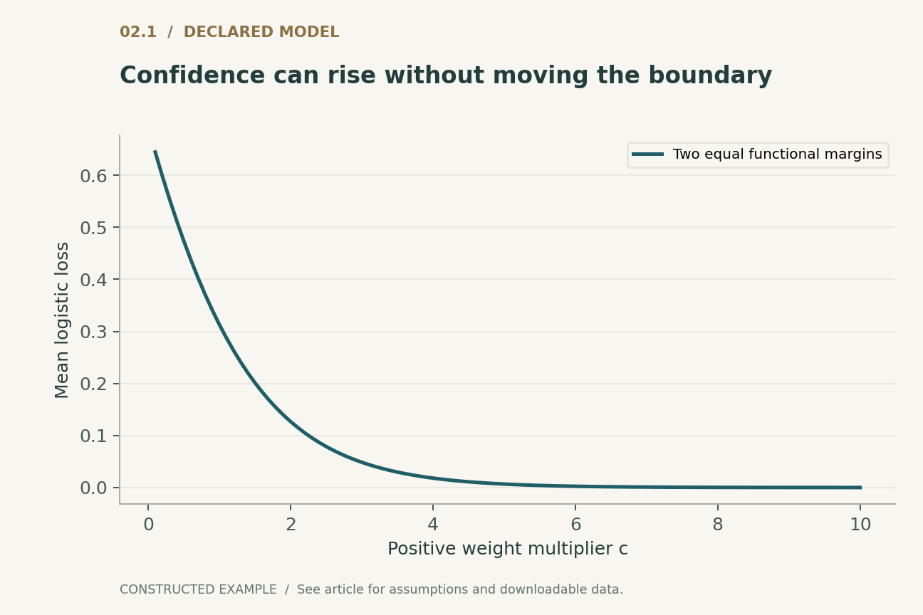
For binary labels y in {-1,1}, logistic loss is log(1+exp(-y w dot x)). Replace w by c w with c>0. The sign of every prediction is unchanged. If the smallest signed score is positive, each loss term decreases as c grows and tends to zero. Meanwhile the norm grows linearly in c, and the decision boundary remains fixed.
The normalized margin divides signed score by the norm of w, so it is unchanged by this rescaling. Thus falling loss can mean only increasing confidence in an unchanged geometry. It can also accompany a changing direction; loss alone cannot tell which. A trace that records loss, norm, normalized minimum margin, and classification error makes these alternatives distinguishable. This is a diagnostic recommendation derived directly from the definitions.
4. An exact two-constraint example
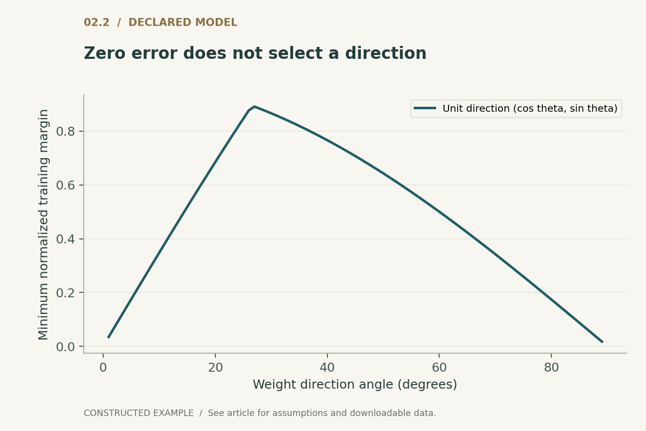
Take two signed feature vectors z1=(1,0) and z2=(0,2), where a signed feature means y times x. The unit functional-margin constraints become w1>=1 and w2>=1/2. Minimizing the squared Euclidean norm subject to those constraints gives w=(1,1/2), since increasing either coordinate only increases the objective. Its normalized minimum margin is 2/sqrt(5).
A direction proportional to (1,1) also classifies both observations correctly, but its minimum normalized margin is 1/sqrt(2). Both have zero training error. At equal norm they have different minimum scores, and after arbitrary positive rescaling both can achieve extremely small logistic loss. This construction isolates the information discarded by the zero-error metric without relying on an unreported dataset or a trained network.
5. Why a slow direction can hide behind fast loss
Once all scores are large and positive, logistic gradients weight lower-margin observations much more strongly than higher-margin ones. This follows from the derivative, whose magnitude is 1/(1+exp(m)) for signed score m. In our two-coordinate example, gradient descent updates the coordinates at different rates because both their feature magnitudes and their current scores differ.
As the parameters grow, absolute updates shrink. The classifier can therefore look stationary by a loss-based threshold while its normalized direction still changes. The supplied finite run illustrates this separation but does not estimate an asymptotic convergence rate from a short trajectory. A rate claim would require either the relevant theorem with its assumptions or an experimental design able to distinguish competing asymptotic forms over a justified range.
6. Coordinate changes modify Euclidean optimization
Let w=A theta for an invertible diagonal matrix A. The represented linear functions are unchanged because every w still has a corresponding theta. A Euclidean gradient step in theta induces a step in w preconditioned by A A transpose. Consequently the trajectory in function space depends on the coordinate system even though representational capacity is identical.
A minimum theta-norm constraint corresponds to an ellipsoidal norm in w. This observation does not assert that every optimizer necessarily converges to that minimum; it identifies which geometry a norm-based conclusion would refer to. Our check compares a direct w update with an A-parameterized update at the same represented function. The gradients are related by the chain rule, and the next functions generally differ. That is a finite, reproducible counterexample to parameterization invariance of ordinary gradient descent.
7. An outlier can determine the geometric buffer
The hard-margin construction gives decisive influence to constraints nearest the separating boundary. Add a signed point epsilon times (1,0) to the example. Its constraint requires w1>=1/epsilon. As epsilon approaches zero, the minimum-norm solution rotates toward the first axis and its norm increases. Every finite positive epsilon still permits perfect classification.
This is not a statement that all rare examples are noise or should be removed. A rare point can represent an important population. The example instead shows that maximizing an empirical geometric margin is conditional on the observations, labels, and feature scaling. If a mislabeled or corrupted point changes separability, the problem itself changes. Data provenance and uncertainty about labels therefore belong in any interpretation of an optimizer's apparent bias.
8. Nonseparability changes the question
Place two identical feature vectors in a dataset with opposite labels. No deterministic homogeneous linear classifier can give both positive signed scores. For their isolated logistic contribution, making the magnitude arbitrarily large worsens one term while improving the other. The loss is minimized at zero score for that contradictory pair.
A larger dataset may contain both contradictory structure and directions that can still separate a subset. The nonseparable analysis of Ji and Telgarsky is relevant because it avoids forcing such data into an all-or-nothing separability story. In this article we check only the symmetric contradictory pair and explain its finite optimum. We do not infer the full decomposition of a realistic dataset from a loss curve or from a low training error. [2]
9. Generalization is an additional inference
A large empirical margin can be useful only relative to a defined feature scale, hypothesis class, and sampling model. If inputs are rescaled arbitrarily, a raw margin can change without any new evidence about unseen labels. If a representation is selected after examining a test set, a margin measured in that representation no longer has the interpretation of a predeclared evaluation.
Even a correct theorem about optimization does not identify the population distribution. To assess generalization, keep a genuinely held-out set, evaluate subgroup and distributional behavior, and distinguish probability calibration from label accuracy. Our constructed example deliberately has no population labels outside its two constraints. It would be mathematically unjustified to assign a test-accuracy advantage to one direction merely because its training margin is larger.
10. A falsifiable study of bias
A proposed experiment should state the predicted limiting object before training: a direction in input space, a norm in parameter space, or a function-space classifier. It should then record the quantities needed to compare the trained model with that object. For small problems, an independently solved constrained optimization problem is a useful reference; for nonlinear networks, an unverified solver output is itself an uncertainty.
The companion examples test exact constraints, norm invariance under positive scaling, the chain-rule preconditioning identity, and the contradictory-pair optimum. They expose how conclusions can fail when an assumption changes. They are intentionally finite. The defensible outcome is not that implicit bias solves generalization, but that optimization selects a geometry which must be named, measured, and separated from the fact of fitting labels.
11. Stopping rules are part of the scientific object
Two training runs with the same optimizer and initialization but different termination rules need not instantiate the same practical claim. A loss threshold favors a confidence scale; a fixed step budget favors a particular point on the directional trajectory; a validation rule introduces another sample and an additional selection procedure. None is intrinsically wrong, but combining their results under one label obscures the comparison.
A report should state whether the chosen checkpoint minimizes validation loss, maximizes validation accuracy, or merely completes a fixed schedule. It should retain the checkpoint trajectory so that a claimed margin improvement can be inspected after the decision rule is fixed. This is especially important when validation loss rises as scores become more confident: a change in probability quality and a change in classification geometry need not have the same sign.
12. A margin is not a probability estimate
Positive scaling leaves the decision boundary fixed but changes logistic probabilities toward zero or one. If the true conditional probability at a particular input is neither endpoint, sufficiently large confidence can worsen its expected logarithmic score even while its predicted label remains correct. The geometric selection problem and the probabilistic estimation problem must therefore be evaluated with different observables.
Executed locally · Bounded scope
Margins, coordinate changes, and contradictory labels
Finite two-constraint geometry, explicit gradient steps and 101 contradictory-pair scores. Finite descent is not proof of the cited asymptotic theorems.
116 assertions passed. These checks validate the supplied example, not the cited systems.
Inspect the recorded witness
{
  "maximum_margin": 0.8944271909999159,
  "trajectory_step_loss_margin": [
    [
      1,
      0.5533380097486379,
      0.4472135954999579
    ],
    [
      10,
      0.2114391196724853,
      0.6472679469278612
    ],
    [
      100,
      0.02618021290683939,
      0.8076515825626189
    ],
    [
      1000,
      0.002528703690596741,
      0.8472075680971195
    ],
    [
      10000,
      0.00025045209849889,
      0.8617419583557351
    ]
  ],
  "direct_gradient": [
    -0.16590611391591695,
    -0.31002551887238755
  ]
}
Example runner · Model loader · Training models · Representation models · Generation models · Reliability modelsRead the complete check results
A declared analytical model
Four equations, explicit assumptions
(1) Binary homogeneous linear logistic loss; no explicit penalty or bias coordinate unless included in x.
(2) Normalized empirical margin is scale invariant for nonzero w.
(3) Exact minimum-norm solution for the article's two signed vectors; not a general deep-network solution.
(4) One Euclidean gradient step in theta; A is fixed and invertible.
Constructed examples · Reproducible data
Inspect the quantitative argument
These curves are calculated from the declared models. They are not observations from the cited studies. Every figure includes its numeric data and vector version.


Which evidence answers which question?
| Observation | What it identifies | What it does not identify |
|---|---|---|
| Zero classification error | Signs on training points | Direction or calibration |
| Decreasing logistic loss | Improving average training score objective | A changing boundary |
| Large normalized margin | Geometry in a specified norm | Population labels or causal invariance |
A proposed validation protocol
This is a proposed evaluation design. No production-system or hardware benchmark was performed. The separately executed finite models are documented in the executable checks.
- Fix feature scaling, labels, loss normalization and parameterization.
- Solve a small reference margin problem independently of gradient descent.
- Log error, loss, norm, direction and normalized margin at each checkpoint.
- Repeat with a coordinate transformation that preserves represented functions.
- Introduce a declared contradictory pair and inspect changed behavior.
- Report the stopping rule and keep test evaluation separate from checkpoint selection.
What the primary sources establish
Daniel Soudry, Elad Hoffer, Mor Shpigel Nacson et al. · 2018 [1]
Contribution. Characterizes max-margin directional behavior for separable homogeneous linear predictors under stated gradient-descent conditions.
Boundary. This is not a blanket theorem for arbitrary finite nonlinear networks.
Source locator. Primary paper, Section 2 and main directional convergence theorem.
Ziwei Ji, Matus Telgarsky · 2019 [2]
Contribution. Analyzes logistic-gradient behavior when data are not completely separable.
Boundary. A separable ray and bounded component require the paper's precise decomposition.
Source locator. Primary PMLR abstract and theorem framework.
Lénaïc Chizat, Francis Bach · 2020 [3]
Contribution. Connects infinite-width two-layer training to a function-space margin.
Boundary. The limiting function geometry and training assumptions differ from the finite linear example.
Source locator. Primary PMLR abstract; infinite-width and homogeneous-activation formulation.
Limits of this analysis
- The worked dataset contains only two signed constraints and has no assigned test population.
- Finite trajectories do not prove asymptotic directional convergence.
- The nonlinear reference concerns an idealized infinite-width setting.
- Margins depend on feature scaling and the chosen norm.
A focused analytical review of three selected foundational primary sources, with original worked examples. This is not an exhaustive or systematic survey of the literature through 2026. Source access and version notes are recorded with the bibliography.
Questions that would change the conclusion
- Which finite-width diagnostics best distinguish a function-space margin from a parameter-space proxy?
- How does a data-dependent stopping rule change the practical bias being measured?
- When do label uncertainty and feature rescaling dominate the optimizer's margin preference?
References
- Daniel Soudry, Elad Hoffer, Mor Shpigel Nacson et al.. The Implicit Bias of Gradient Descent on Separable Data. Journal of Machine Learning Research 19(70) (2018). Primary source.
- Ziwei Ji, Matus Telgarsky. The implicit bias of gradient descent on nonseparable data. Proceedings of the Thirty-Second Conference on Learning Theory, PMLR 99 (2019). Primary source.
- Lénaïc Chizat, Francis Bach. Implicit Bias of Gradient Descent for Wide Two-layer Neural Networks Trained with the Logistic Loss. Proceedings of Thirty Third Conference on Learning Theory, PMLR 125 (2020). Primary source.
Source [1] access. JMLR record and primary PDF introduction/theorem context inspected; full proof not independently audited.
Source [2] access. Primary bibliographic record and abstract inspected; no exhaustive full-text or supplementary-material audit.
Source [3] access. Primary bibliographic record and abstract inspected; no exhaustive full-text or supplementary-material audit.
Bibliographic identities were checked against primary publisher and author records. Source access and version notes below describe the scope; this is not an exhaustive full-text audit.
Authorship and provenance
Written and technically self-reviewed by Codex (AI). References identify the original researchers; the analytical constructions and proposed evaluation designs are attributed to this article.
Covers are conceptual ImageGen illustrations. Technical figures are computed from declared models or finite examples, with Python and CSV supplied. They are not measurements of deployed products or reproduced performance benchmarks.
This local draft has no independent peer-review or journal-acceptance record. Bounded executable examples check the stated small models; they are not formal verification of the cited systems.