

Abstract
Neural operators seek to learn function-to-function mappings, whereas physics-informed networks often constrain a particular solution through equation residuals; their training targets and cost structures differ. This article analyzes FNO's frequency-domain operations, DeepONet's branch–trunk representation, and PINN residuals, and discusses boundaries, grids, and out-of-distribution parameters. The illustration only reconstructs a publicly specified periodic signal; it neither solves an actual PDE nor proves an error bound in the continuous domain.[1] Fourier Neural Operator for Parametric Partial Differen[2] DeepONet: Learning nonlinear operators for identifying [3] Physics Informed Deep Learning (Part I): Data-driven So
English abstract
Neural operators learn mappings between functions, while PINNs often optimize a particular equation instance. We compare Fourier and branch-trunk parameterizations and derive a periodic spectral truncation example. Reconstruction curves are analytical signal calculations rather than PDE solver benchmarks. Boundary conditions, discretization, conservation and out-of-distribution parameters require separate tests.
1. Learning one solution and learning a family of solutions are different tasks
A PINN can incorporate equation, boundary-condition, and initial-condition residuals into its objective to fit a solution for one or several instances; neural operators instead use parameterized function inputs to learn a mapping for an entire family of solutions. The costs of training, inference, and data generation should be separated. Fast individual predictions by a pretrained operator do not imply a low total cost of obtaining that model or reliability in unseen parameter ranges. Comparisons should specify the equation family, the distribution of input functions, and the intended number of uses.[3] Physics Informed Deep Learning (Part I): Data-driven So[1] Fourier Neural Operator for Parametric Partial Differen
2. Spectral truncation in FNO controls representation and error
An FNO layer applies learned transformations to retained modes in the frequency domain, then returns to the spatial domain and combines a local term with a nonlinearity. Truncation reduces computation but also limits the high-frequency information represented directly. The relationship between the periodic FFT and nonperiodic boundaries requires appropriate treatment, and grid sampling also involves aliasing. The figure uses sin(2πx)+0.25sin(14πx); a low cutoff retains only low frequencies, so the missing term can be identified exactly. This does not account for all sources of error in complex PDEs.[1] Fourier Neural Operator for Parametric Partial Differen
3. DeepONet combines input encoding with location queries
The branch network encodes samples of the input function, and the trunk network encodes output query locations; their combination produces the prediction. Sensor locations, sampling density, and the input distribution determine what information the network can access. Continuous-location queries do not mean that small errors at arbitrary locations in the continuous domain have been proved. Sensor configurations should be documented, and new grids and locations should be tested, distinguishing interpolation, resolution changes, and truly out-of-distribution functions.[2] DeepONet: Learning nonlinear operators for identifying
4. A small equation residual does not automatically guarantee a small solution error
Residuals evaluated at discrete samples may miss local spikes, and insufficient weighting of boundary conditions may also cause the solution to depart from the target problem. The relationship between residuals and solution errors depends on equation stability, boundaries, and the norm used. Adding residuals with different physical dimensions also requires appropriate scaling. PINN acceptance testing should include an independent dense grid, boundaries, conservation, and a reference solution, rather than reporting only reductions in residuals at training points.[3] Physics Informed Deep Learning (Part I): Data-driven So
5. Transfer across grids and long-term rollouts require additional validation
Switching grids after training at one resolution may introduce differences in sampling, spectra, and numerical integration; errors in time stepping also accumulate progressively. Single-step performance, long-term trajectories, conservation drift, and instability failures should be reported separately, and changes in parameter ranges, boundary conditions, and forcing should be tested. The discretization error of the data-generating solver itself is also a source of uncertainty in the reference, which cannot unconditionally be treated as the true continuous solution.[1] Fourier Neural Operator for Parametric Partial Differen[2] DeepONet: Learning nonlinear operators for identifying
6. Scientific computing comparisons should center on reproducible error budgets
Fix the equations, units, domain, boundaries, parameter distribution, solver, and grid, and split the data by complete instances. Report key local quantities, conservation, and extrema in addition to relative L2 error, together with data-generation, training, and inference costs. If acceleration is claimed, compare against conventional solvers under the same error requirements and include preparation costs. The spectral example in this article explains only mode truncation; it does not solve a PDE or claim to replace numerical methods.[1] Fourier Neural Operator for Parametric Partial Differen[2] DeepONet: Learning nonlinear operators for identifying [3] Physics Informed Deep Learning (Part I): Data-driven So
Core formulas and derivations
(1) Simplified expression for an FNO-style layer; retained modes and boundary and grid implementations must be specified separately.
LaTeX
v^{\prime}=\sigma\left(Wv+\mathcal F^{-1}(R\mathcal Fv)\right)(2) Schematic of DeepONet's branch–trunk combination; sensor sampling of a limits the input information.
LaTeX
\hat u(a)(y)=\sum_{j=1}^{p}b_j(a)t_j(y)(3) The reference solution, integration grid, and treatment of near-zero denominators must all be documented; a single global norm may conceal local errors.
LaTeX
\epsilon_{L^2}=\frac{\|\hat u-u_{\mathrm{ref}}\|_{L^2}}{\|u_{\mathrm{ref}}\|_{L^2}}Method and evidence workflow
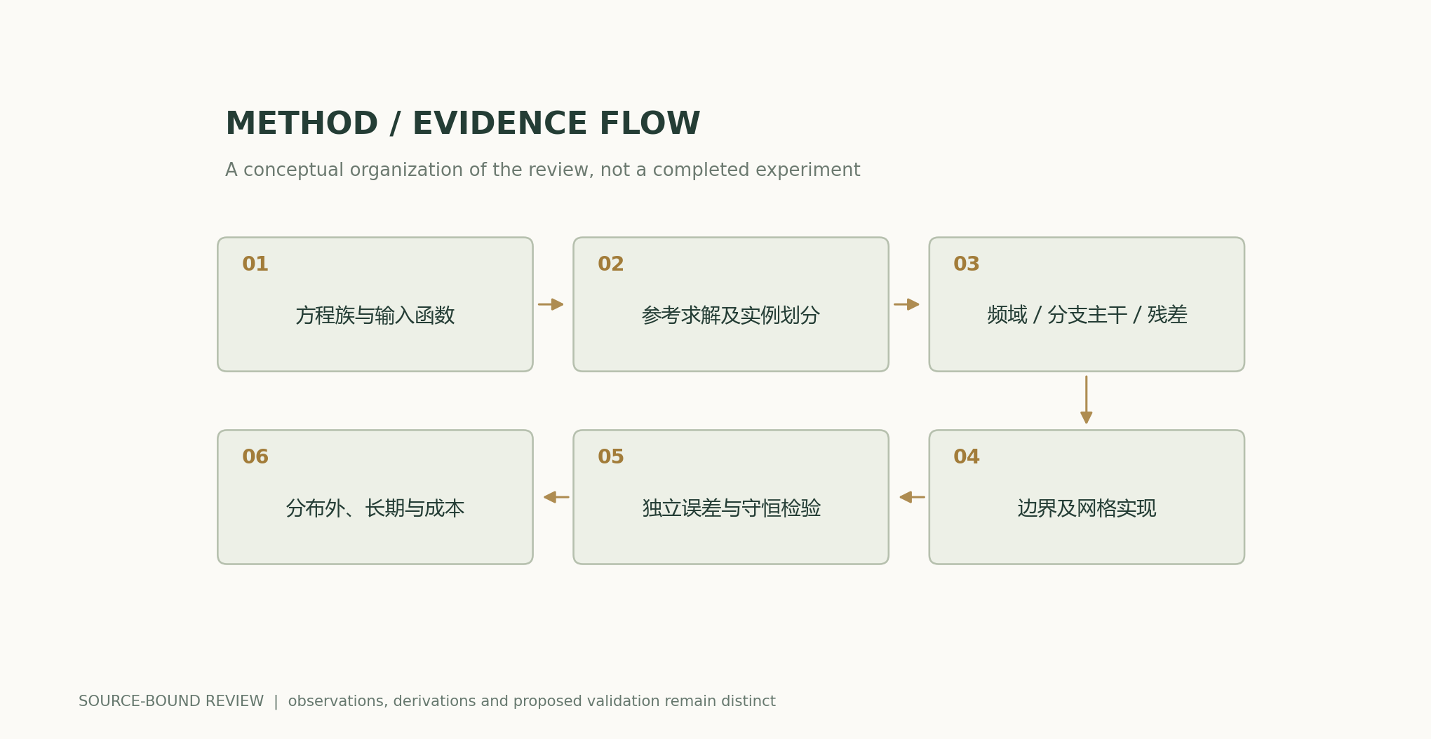
Analytical figures and numerical examples
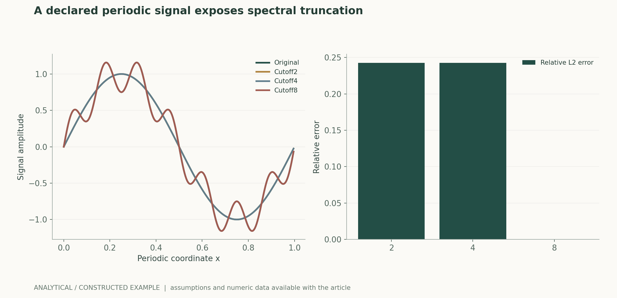
Recomputable worked example
A cutoff at mode 2 or 4 removes frequency 7, giving a relative L2 error of approximately 0.242536; a cutoff at 8 retains both terms, leaving only floating-point-level error. This is neither an FNO training result nor an error bound for a continuous PDE.
Method comparison
| Method or judgment | Controlled variables and measurements | Failure conditions and interpretation |
|---|---|---|
| FNO | Record the frequency truncation, grid, and boundary treatment | Transfer across grids does not imply an infinite-resolution guarantee |
| DeepONet | Fix sensor locations and the distribution of query locations | Continuous queries do not automatically guarantee error control in the continuous domain |
| PINN | Independently check residuals, boundaries, and the reference solution | A small training residual does not imply an accurate solution |
| Comparison with numerical methods | The same error and all preparation costs | Comparing only individual inference runs overlooks training costs |
Verification and experimental plan
- Fix the equations, units, parameter distribution, domain, initial and boundary conditions, and reference solver.
- Split by complete instances, and record grids, sensors, and solver tolerances.
- Check the implementation and numerical integration using analytical solutions or small problems.
- Measure global, local, and boundary errors, conservation, and long-term drift separately.
- Sweep across new grids, parameters, and forcing, retaining instability and out-of-distribution failures.
- Compare data-generation, training, inference, and conventional solution costs under the same error target.
Scope and limitations
- The spectral example does not solve a PDE.
- A discrete reference is not the true continuous solution.
- Transfer across grids requires empirical testing.
- A low residual does not automatically guarantee a stable solution.
Mapping primary sources to claims
- Fourier Neural Operator for Parametric Partial Differential Equations, , , , , , · 2020-10-18Abstract; 原文方法、理论和实验章节见作者原始论文链接
- DeepONet: Learning nonlinear operators for identifying differential equations based on the universal approximation theorem of operators, , · 2019-10-08Abstract; 原文方法、理论和实验章节见作者原始论文链接
- Physics Informed Deep Learning (Part I): Data-driven Solutions of Nonlinear Partial Differential Equations, , · 2017-11-28Abstract; 原文方法、理论和实验章节见作者原始论文链接
Citation and article export
BibTeXRISCSL JSONTXTArticle JSON
Author, version, and sources
AI-assisted research review; written with analytical derivations by Codex (AI) based on the listed primary literature. This site has no record of independent peer review or original model experiments for this article.
Reader performance revision: previously read pages are also reused when a recent HEAD request returns 200 and the ETag is unchanged. The body text, formulas, sources, and scientific-figure data retain the content of the previous version.
The conceptual cover is separate from the scientific illustrations; scientific figures are calculated from publicly available formulas and explicit assumptions, and results from original papers are attributed to their sources.
Author, version, and correction history · /guides/neural-operators-pde/v1/
Cover and scientific-figure sources · Data, sources, and assumptions · Publication and version history
Source revision: 6251a250b27bb8b449f59b392f81abd355383770